Frequently Asked Questions
Here, we will keep some FAQs before they are published to the main documentation.
Global Material data
Copy any material to Global through the Materials tab
Or copy between computers those materials ar files.
They are stored
C:\Users\%username%\AppData\Roaming\Trafolo\materials
Converting Gauss to Teslas
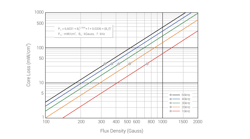
Given in kGauss and kHz:
We don't have a way to export this macro.
Converted to Teslas an Hz
We don't have a way to export this macro.
For the example above, new values are
We don't have a way to export this macro.
We don't have a way to export this macro.
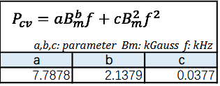
We don't have a way to export this macro.
We don't have a way to export this macro.
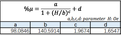
We don't have a way to export this macro.
We don't have a way to export this macro.
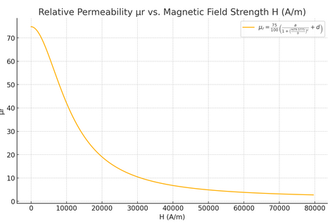
This data is crap - the BH curve is always ascending function - both values only go up.
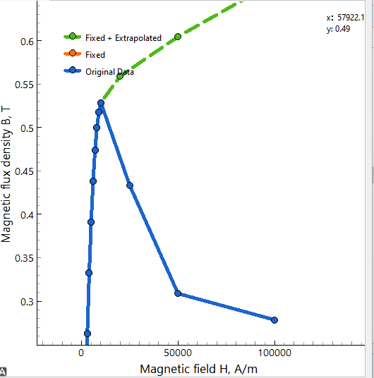
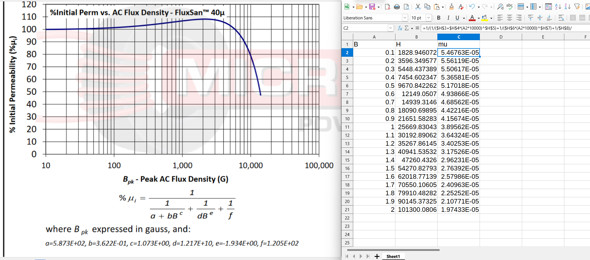
Obtaining BH for Micrometals
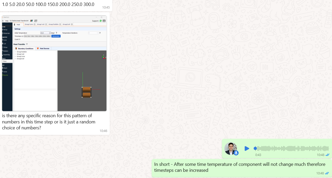
Transient temperature
IGSE (Improved Generalized Steinmetz Equation) vs GSE
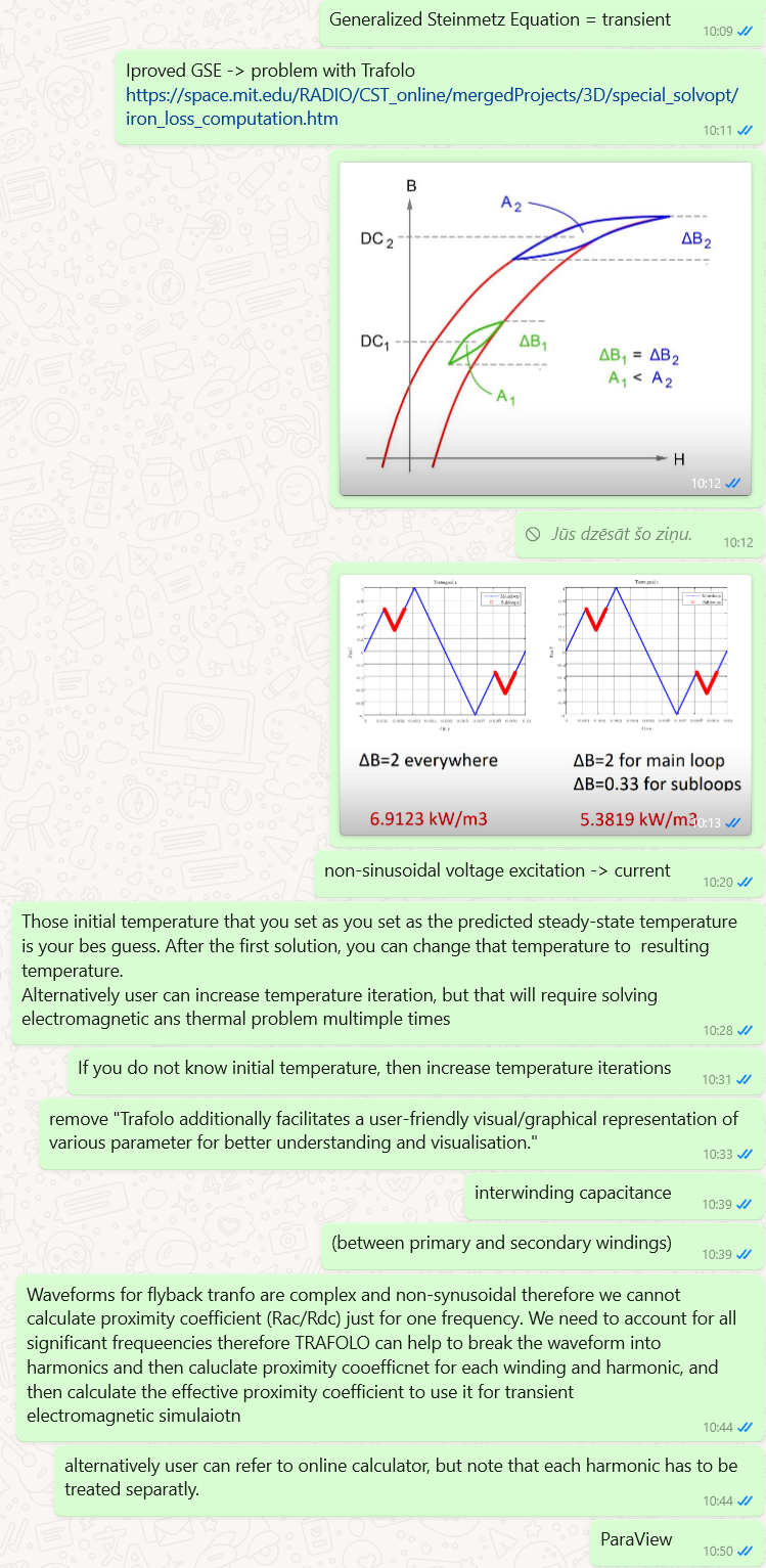
Effective Rac/Rdc coefficient
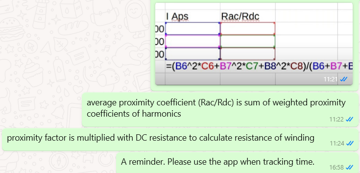
Fill factor
Definition: The total cross-section of conductor material divided by the cross-section of geometry.
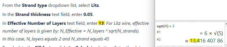
The effective number of layers
There is no consensus whether we need to round numbers or not. Dowell calculator on the Web accepts only integers, while the equation can be used with floating numbers. Engineers often round those numbers to read values from graphs. I suppose it relates to the "old way of doing things".
Depending on case, the difference usually is <5%.
Number of layers, strands, and parallel wires
Secondary (orange)
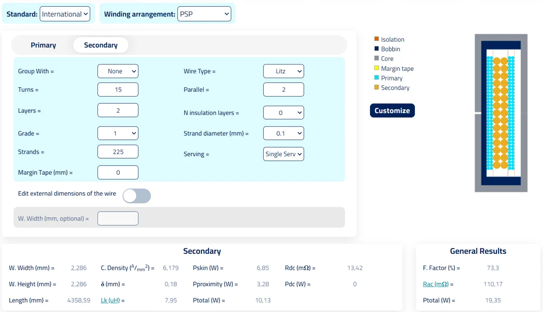
It has 15 turns, each turn consists of 2 parallel wires (bifilar). For this reason there are 30 wires shown in the picture.
The wire is wound in 2 layers, and each wire consists of 225 strands.
WInding is interleaved by primary windings on both sides, interleavingCoefficient = 0.5 meaning that the effective number of layers will be reduces by half. When the winding is placed between two other windings, it is considered interleaved.
Neff = Nlayers * interleavingCoefficient *sqrt(Nstrands) = 2 * 0.5 * sqrt(225) = 15
Primary (blue)
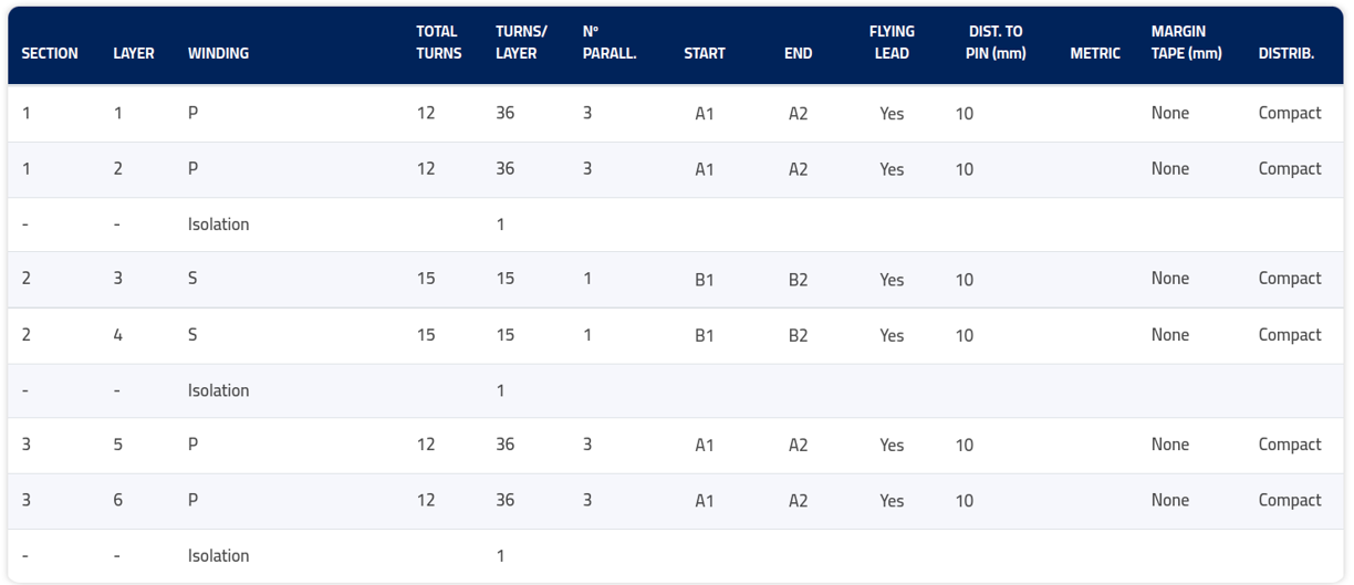
It has 2 windings - one inside, another outside. We should treat those as separate geometries and separate windings that are just connected in series with circuits.
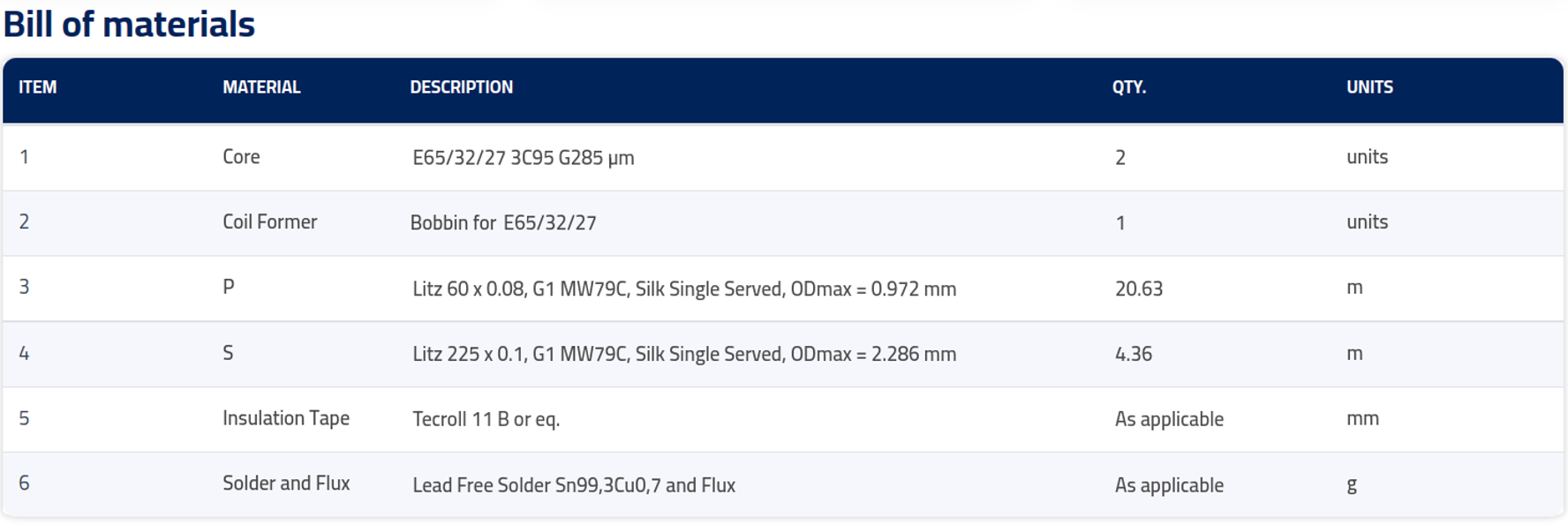
Each winding has 2*12=24 turns. Each turn consists of 3 parallel wires (trifilar). The wire is wound in 2 layers. Each litz wire comprising 60 strands (see bill of materials above).
For this reason, 2*12*3 = 72 wires are seen in the picture for each primary winding.
Primary windings are not interleaved as they are not placed between other windings. It means that interleavingCoefficient = 1 and we can skip it.
Neff = Nlayers *sqrt(Nstrands) = 2 * sqrt(60) = 15.5
Terminals
One conductor can have multiple possitive/negatie terminals
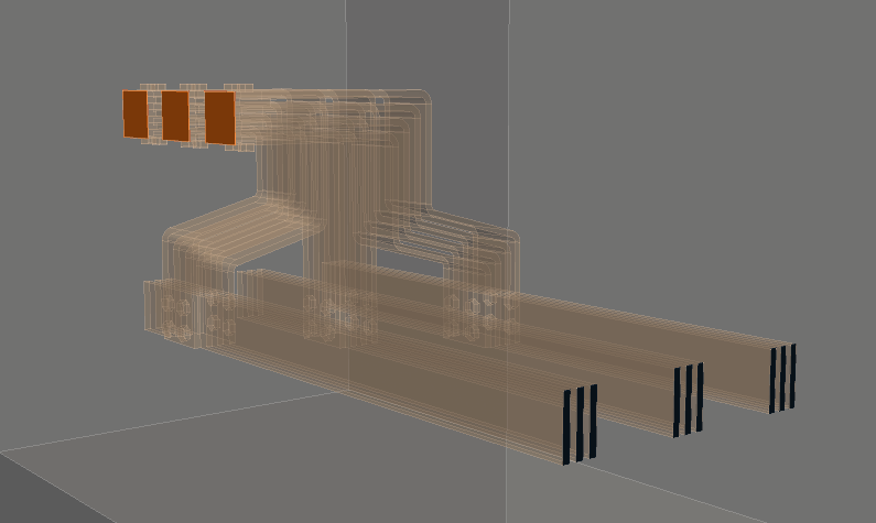
Heat transfer coefficient values
When geometry is assembled again, the heat transfer coefficient values are reset to the default values of 5 W/m2/k. The same is the case with meshing and terminals in Elmag.
High aspect ratio & convergence
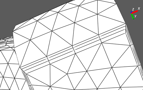
High aspect ratio may reduce convergence rate. At this moment, we do not inform user about bad convergence/divergence.
You can check that in the terminal. We set 1e-9 residual by default.

High aspect ratio might also affect accuracy, but that mostly depends on the field gradient and its direction. To get accurate results, we need to have finer mesh in the direction of field gradients.
Boundary mesh
You will see them when looking from the terminal side. For other non-coils you will not see then in the preview.
This is pic from High Frequency Inductor template
More advanced thing to see the entire mesh after it is generated:
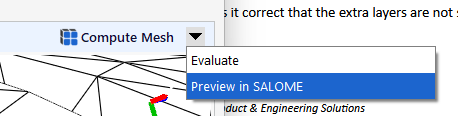
Then switch to Mesh module
Enable mesh
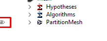
Right click on the mesh -> Clip. Once you clip, you should see the inner elements.
Accuracy of inductance calculations
- Add bobbin between coils, and set material as air.
- And apply finer mesh to that bobbin or even boundary layers.
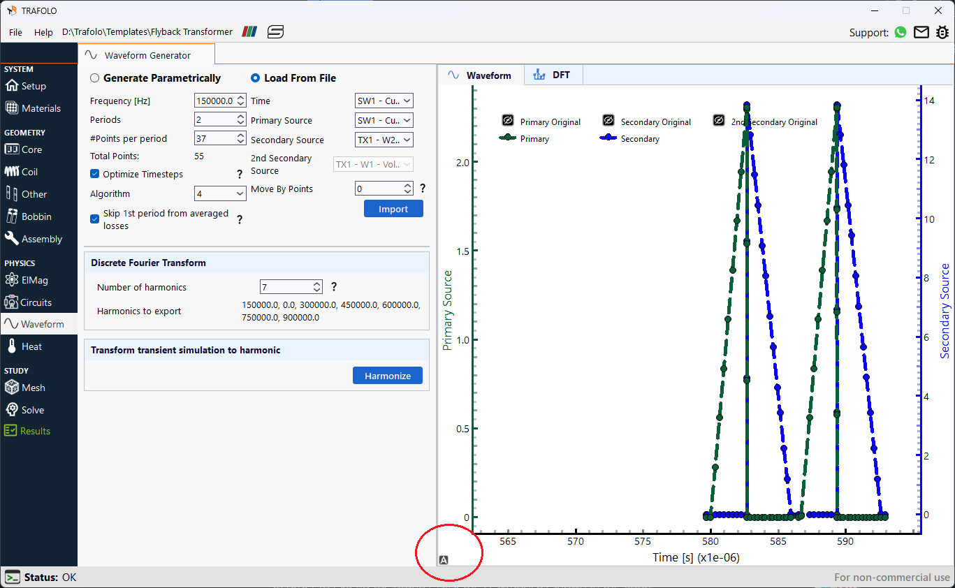
Rescaling graphs
To extend the graphs, click the A symbol shown in the figure below.
Determining Magnetic Flux in the Core
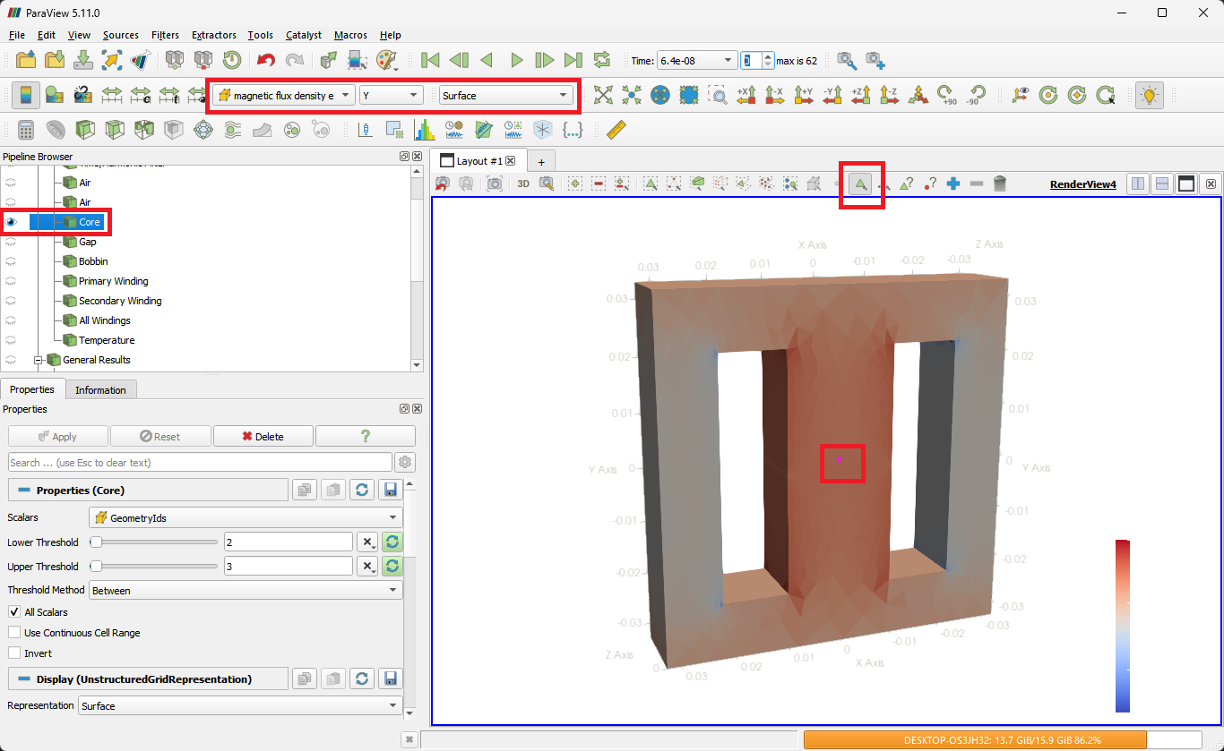
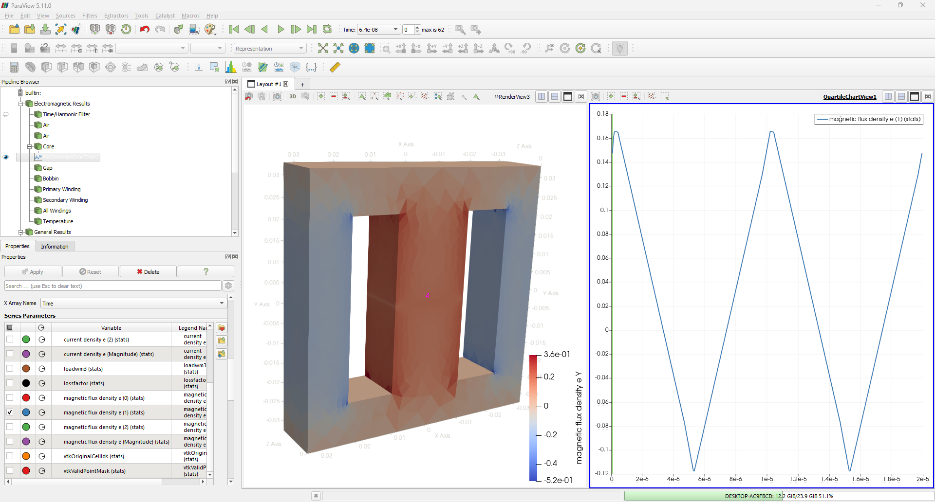
The magnetic flux density distribution can be visualized in ParaView, enabling precise examination of flux density variations at any point over time. Given that the maximum flux density is typically found in the central limb of the core, an element/cell on this limb is selected for analysis by plotting.
To visualize the magnetic flux density change over time for the central limb, navigate to the Pipeline Browser and make the Core visible under Electromagnetic Results by clicking the eye icon. In the Attribute toolbar, select magnetic flux density e from the first dropdown and Y from the second dropdown. Next, from the RenderView toolbar, click on Interactive Select Cells and choose an element on the central limb for which the field values are to be plotted. In the Menu bar, click on Filters, then search for and apply Plot Selection Over Time.In the Properties tab, click Copy Active Selection, then click Apply. Finally, navigate to Series Parameters, check the Magnetic Flux Density e (1) (stats) box, and uncheck all other boxes. The plot will be displayed.
Why we prefer to set currents instead of voltages
When we set voltages on both primary and secondary, the current is only limited by the impedance of the transformer windings. The model does not know that the secondary side has some load that further reduces the current flow. As a result, you will get high currents.
If we set voltage, then software calculates current and vice versa.
If it is transient waveform then we should be aware of inrush currents
https://www.linkedin.com/pulse/core-losses-whats-point-using-current-instead-voltage-8-trafolo-fbajf
We usually calculate magnetizing and leakage inductances, resistances of windings and then simulate equivalent circuit model. Then we take waveforms and feed into FEM to calculate losses etc.
Why do primary and secondary windings share the same ground?
Ground is used for both primary and secondary to set up the reference potential 0. In numerics, the problem must be uniquely defined. Without it, there will be infinite solutions as the voltage drop of 10V could be achieved by voltages on the terminals such as 0 and 10, -5 and 5, -10 and 0. The solver, otherwise, will diverge. We can set any reference potential, but setting 0 is just more convenient. Connecting both primary and secondary to the ground is no problem as the numerical ground has an ideal of 0 resistance, which is not the case in real life.
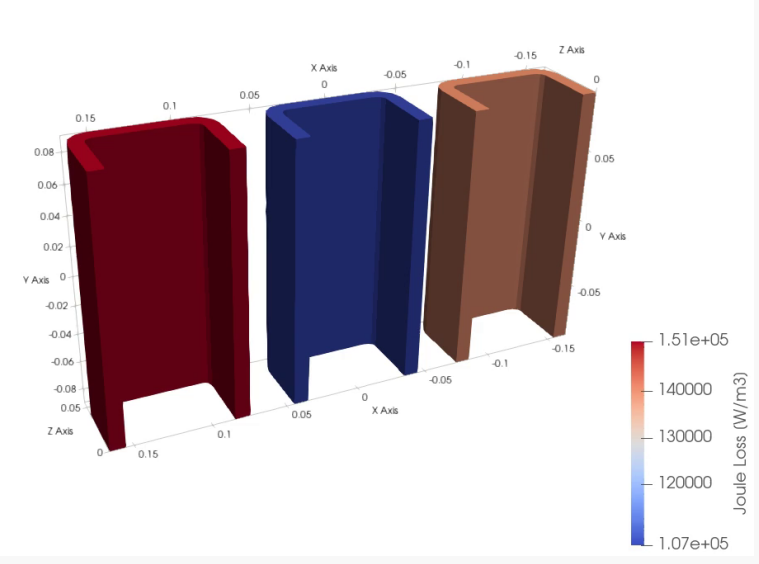
Non-symmetries in 3-phase transformers
Seemingly symmetric case, but having winding losses 5% off between side limbs. This means that current error is sqrt(1+5%)-1 ~ 2.5%.
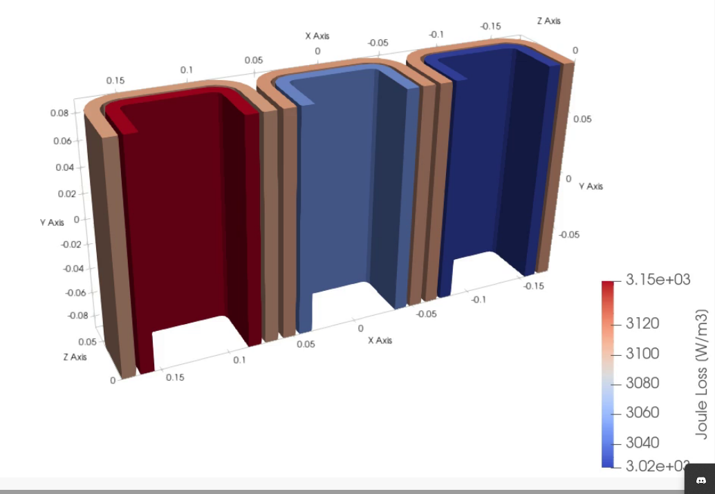
There seems to have no difference in these factors:
- mesh refinement
- swapping phases
- changing BH to const permeability
- removed core
- removed secondary, error became even larger
Building spacers Using bobbin tab
The xg and zg parameters define the lengths of the bobbin walls that need to be cut away to create spacers. Simply put, these parameters represent the distance between the spacer edges.
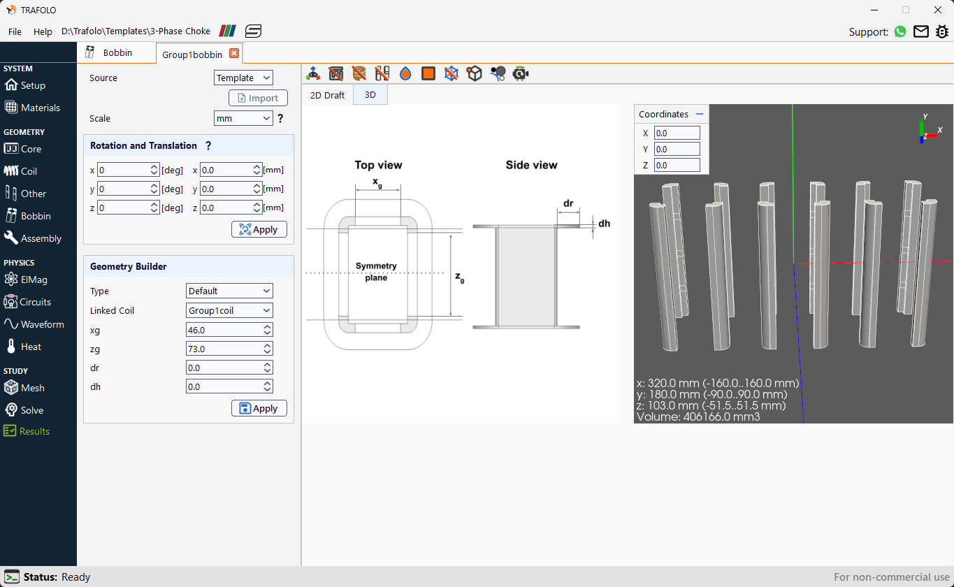
“Linked coil” in Bobbin Geometry
The "linked coil" feature enables the software to automatically generate a bobbin that precisely fits between the core and the coil. By linking the bobbin to the Group1coil winding, the software utilizes the existing dimensions of the core and coil to define the bobbin's geometry accurately. This feature eliminates the need for users to manually input measurements, such as the bobbin's length or thickness.
Mesh Refinement for Accurate Simulation Results
In general, users should perform mesh analysis by starting with a coarse mesh and then refining it iteratively. Initially, a coarse mesh provides a general solution at a lower computational cost. However, regions with high gradients may require finer resolution to capture the physics more accurately.
Refining the mesh in these regions ensures that the solution becomes more precise. This process is repeated until the difference between results from successive simulations becomes negligible or within an acceptable tolerance. At this point, the solution is considered mesh-independent, indicating that further refinement will not lead to significant changes in the results, ensuring accuracy.