Modelling Litz Wire using Homogenization
Introduction
Copper losses in high-frequency magnetic components are predominantly influenced by the skin and proximity effects, which result in non-uniform current distribution and increased AC resistance. Litz wire is commonly used due to its multiple insulated strands to mitigate these losses, which effectively reduce skin effect losses by maintaining a more uniform current distribution. However, proximity effect losses remain challenging, especially in high-frequency environments where magnetic field interactions between adjacent conductors cause further current non-uniformity.
While analytical models like the extension of Dowell's equation onto Litz/stranded wires provide theoretical estimates for these losses, they often fail to capture the complex behaviors observed in practical applications, particularly while dealing with non-uniform magnetic flux distribution. Additionally, circulating currents, which arise from imperfect parallelism and mutual inductance between individual Litz wire strands or bundles, further increase losses. To accurately measure these losses, Finite Element Method (FEM) software can be employed.
However, resolving the skin and proximity effects in each strand requires a fine mesh size—at least three times smaller than the skin depth as a rule of thumb, making the simulations computationally intensive. Therefore, instead of modeling each strand individually, the homogenization technique is employed to simplify the process. To learn more about the method, visit the article in our newsletter.
TRAFOLO significantly enhances simulation efficiency, particularly at high frequencies using homogenization. It simplifies the modeling of litz windings, enabling faster and more manageable simulations while preserving essential accuracy. This approach is especially effective for complex geometries like gapped inductors and transformers, striking an optimal balance between reducing computational effort and maintaining precision.
Model Description
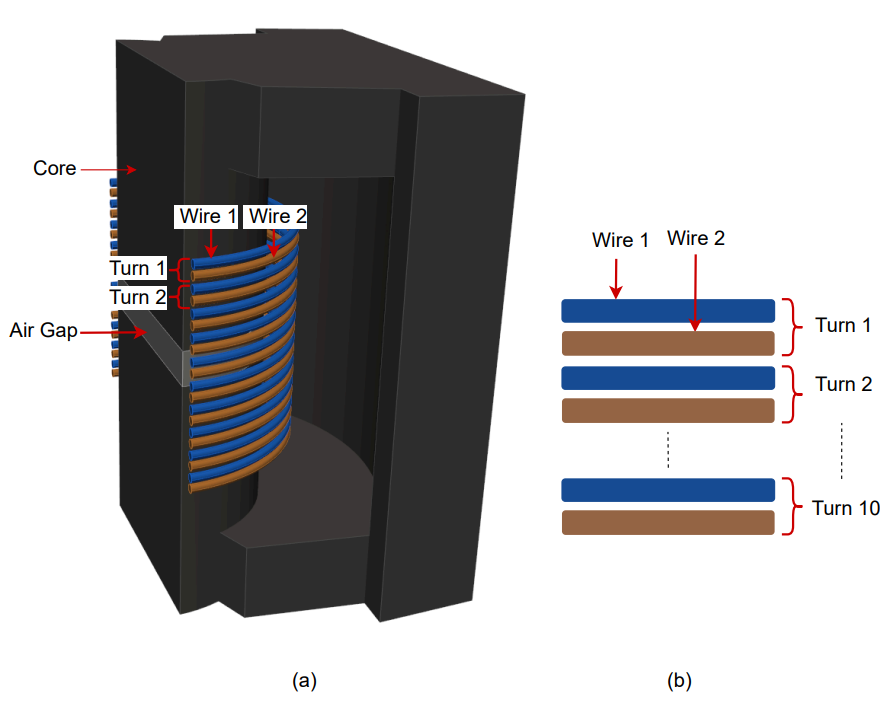
The reactor described in the paper "Analysis of Litz Wire Losses Using Homogenization-Based FEM" by Y. Otomo et al. is being modeled to demonstrate and validate the homogenization technique within TRAFOLO. Although the paper employs a slightly different method for homogenization—using pre-calculated complex permeability via Bessel functions—the core principle of homogenization aligns.
The reactor features a PQ65 core with a 4 mm air gap. We have taken N95 TDK 100C as core material with an initial permeability of 3000. The winding consists of two parallel litz wires, each with 10 turns wound in a single layer, with no twisting between the wires. The litz wire comprises 7 strands, each with a radius of 0.16 mm. The reactor is excited with a 1A input, and its response is analyzed over a frequency range from DC up to 120 kHz (up to 100 kHz in the original paper). The key specifications are summarized in the table below:
| Core type | Core material | Initial permeability | Air gap | Strands/wire | Twist pitch | Strand diameter | Wire length | Turns |
|---|---|---|---|---|---|---|---|---|
| PQ65 | N95 TDK 100C | 3000 | 4 mm | 7 | 20 mm | 0.32 mm | 1000 mm | 10 |
Modeling Instructions
Setup
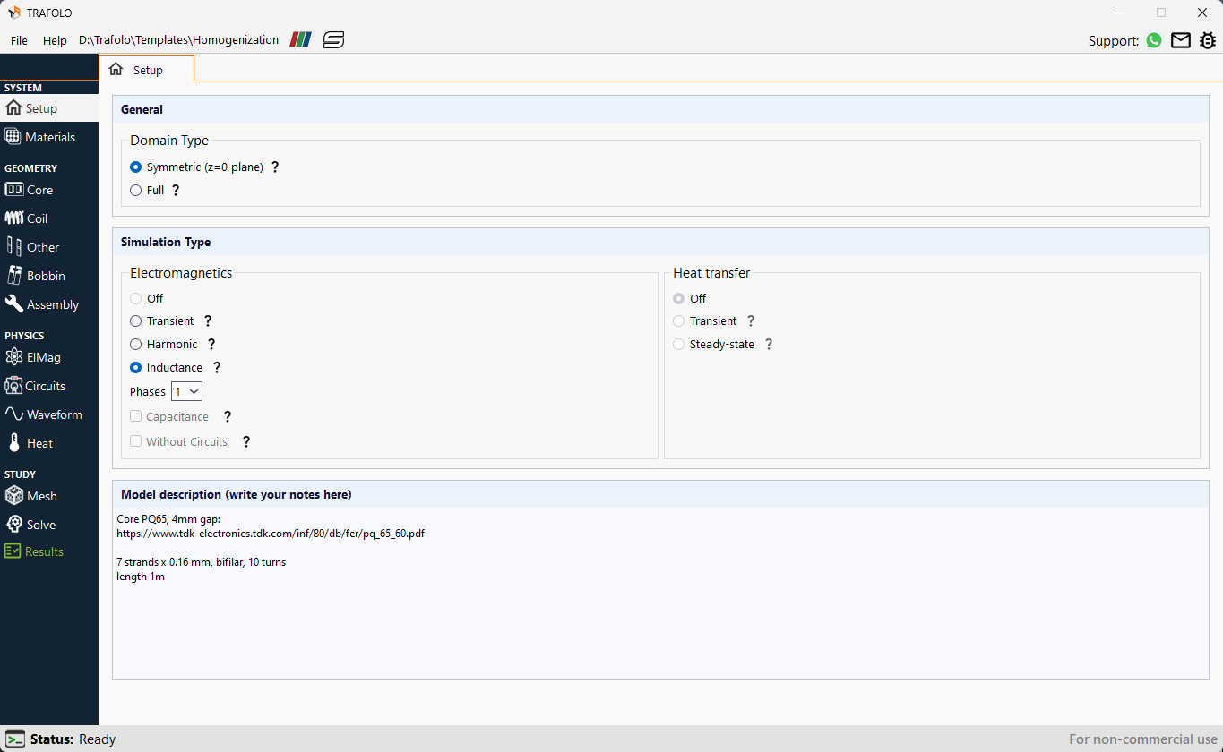
- From the Model Builder, click the Setup tab.
- Locate the General section and set the Domain type as Symmetric (z=0 plane).
This setting is beneficial for models with a plane of symmetry that divides the core and the coil into symmetrical segments. This method ensures that the computed values reflect the complete system despite only modeling a symmetrical section. Subsequently, parameters such as voltage, resistance, losses, inductance, and other related values are appropriately scaled to represent the entire geometry accurately. - In the Simulation Type section, set Electromagnetics to Inductance.
- Heat transfer is disabled by default for inductance simulation.
Materials
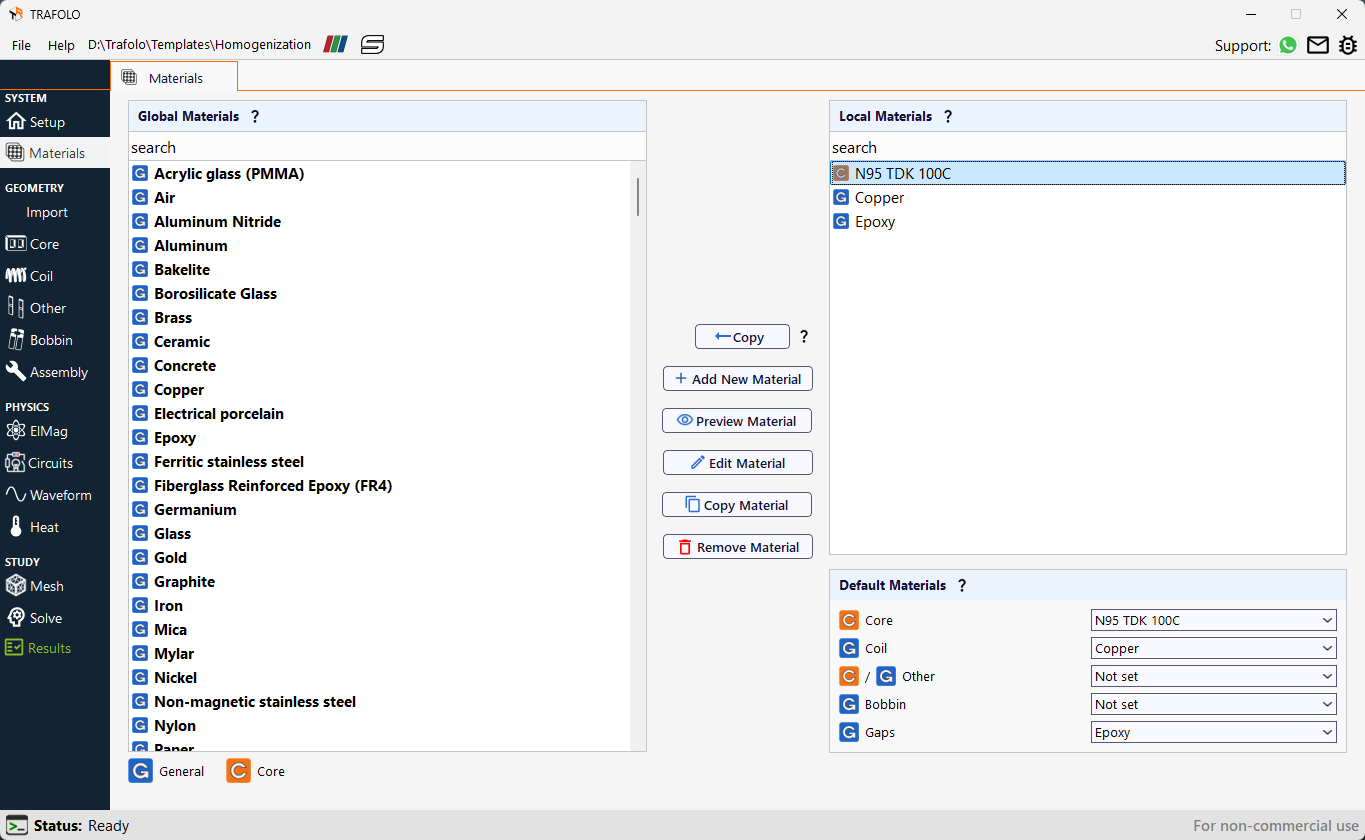
- Select the Materials tab from the Model Builder.
- From the Global Material section, select Copper and click the Copy button.
- Similarly, copy N95 TDK 100C and Epoxy from the Global Materials section to the Local Materials section.
- In the Default Materials section, select the material type for each component from the dropdown list as per the table below:
| Component | Core | Coil | Other | Bobbin | Gaps |
| Material type | N95 TDK 100C | Copper | Not set | Not set | Epoxy |
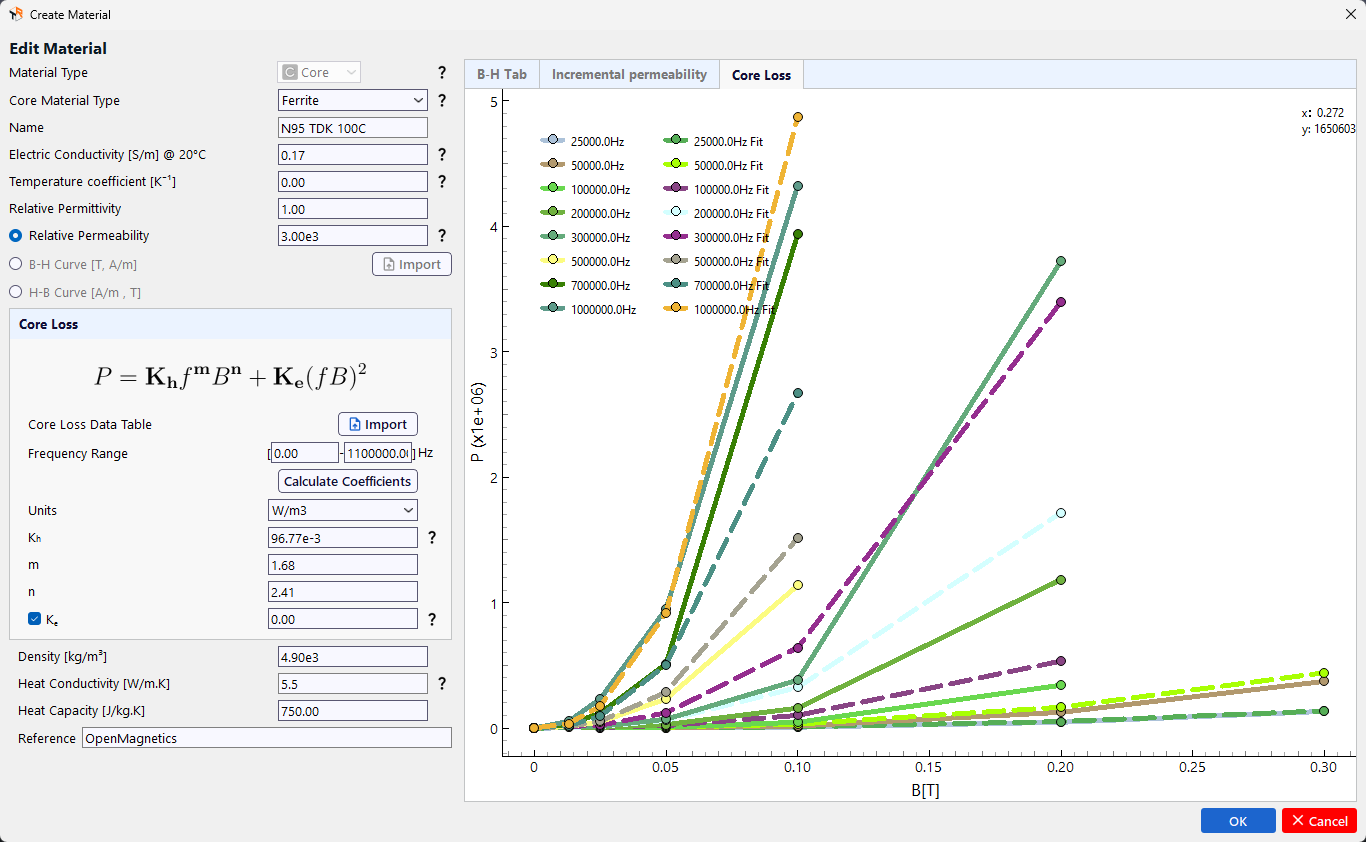
- In the Local Materials section, select N95 TDK 100C and click the Edit Material button.
- In the Edit/Create Material dialog box, mark the Relative Permeability and enter 3000 in the corresponding text field.
Note: Assuming the PQ65 core is made of N95 material, the PQ656 N95 datasheets specify an effective permeability of 2270 and an initial permeability of 3000 (at 25°C). Since the transformer operates at low magnetic flux densities (below 0.02 T) and the air gap is resolved numerically, the initial permeability is appropriate to use. While permeability can vary with temperature, the value at 25°C can be used for simplicity.
Given that the central limb includes an air gap, permeability variations—whether around 1000 or 5000—will have minimal impact on overall performance. 7. Click the Ok button.
Core
- From the Model Builder, click on the Core tab.
- Click the New Group button. The Group1core will be added.
- Click the Open in new tab icon. The Group1core tab will open.
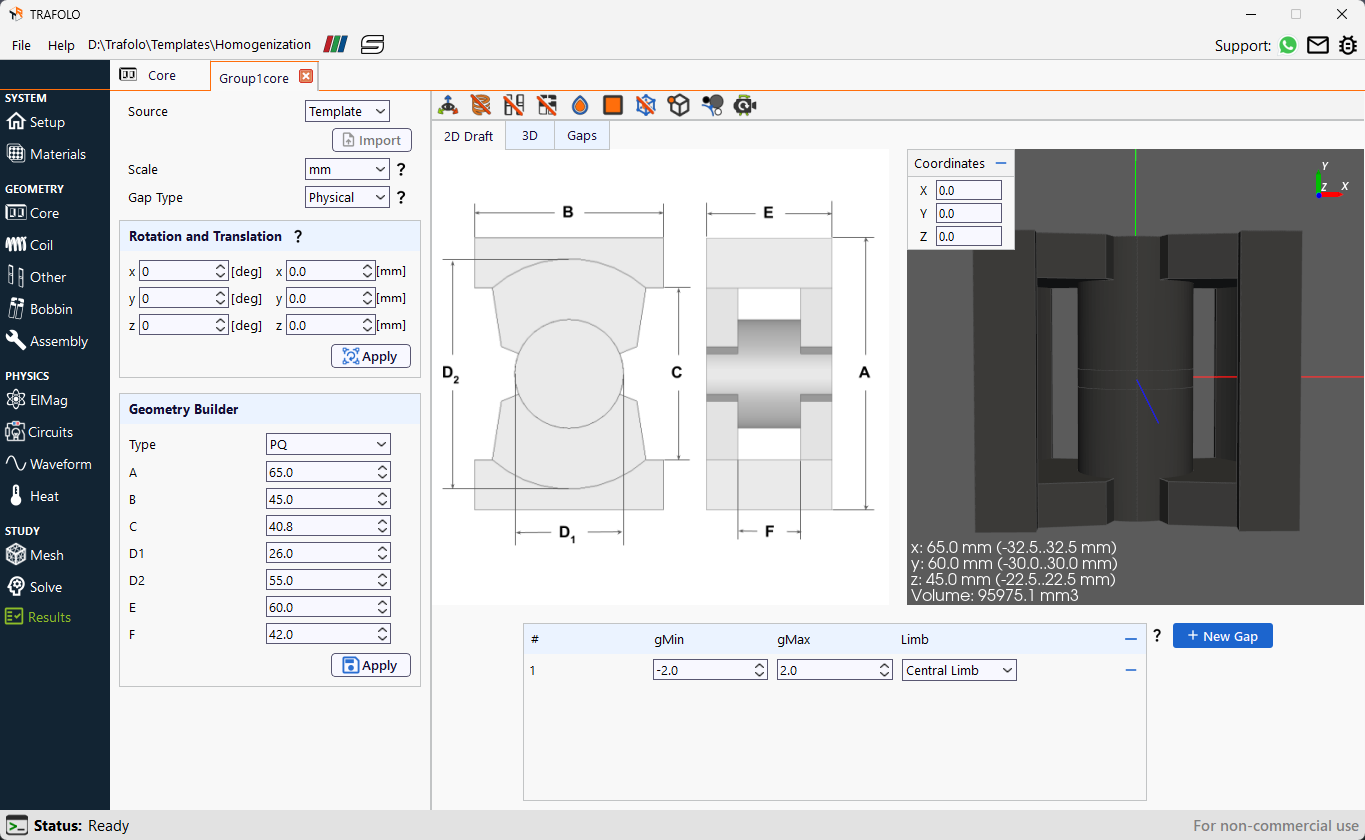
- From the Source dropdown list, select Template.
- From the Scale dropdown list, select mm.
- From the Gap Type dropdown list, select Physical. This will cut the core geometry and create a gap as a separate body with assigned material properties.
- In the Geometry Builder section, set the Type to PQ and enter the dimensions (mm) as per the table below:
| A | B | C | D1 | D2 | E | F |
| 65.0 | 45.0 | 40.8 | 26.0 | 55.0 | 60.0 | 42.0 |
- Click the New Gap button.
- In the gMin and gMax text fields, enter -2.0 and 2.0,respectively.From the Limb dropdown list, select the Central Limb. This will create a gap of 4.0 mm in the central limb of the core.
-
Click the Apply button.
Coil
- From the Model Builder, click on the Coil tab.
- Click the New Group tab. Group1coil will be added.
- Click the Open in new tab icon. The Group1coil tab will open.
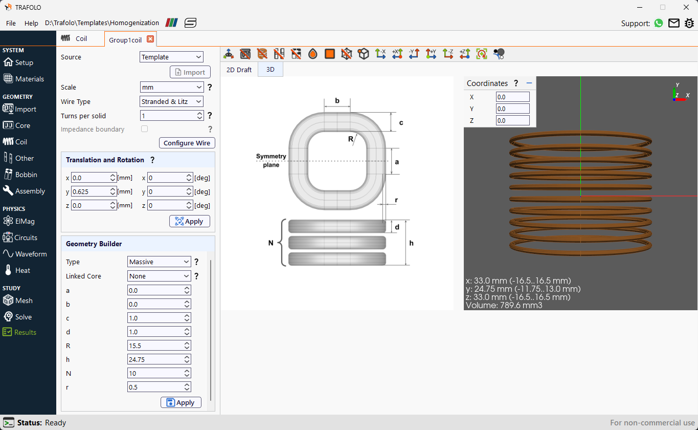
- From the Source dropdown list, select Template.
- From the Scale dropdown list, select mm.
- From the Wire Type dropdown list, select Stranded & Litz wire.
- Set the Turns per solid to 1.
- In the Geometry Builder section, set the Type to Massive and the Linked Core to None.
- Enter the dimensions (mm) according to the table below.
| a | b | c | d | R | h | N | r |
|---|---|---|---|---|---|---|---|
| 0.0 | 0.0 | 1.0 | 1.0 | 15.5 | 24.75 | 10 | 0.5 |
- Click the Apply button.
-
Set the translation along the y-axis to 0.625 mm in the Rotation and Translation section and click the Apply button.
 11. Click the Configure Wire button.
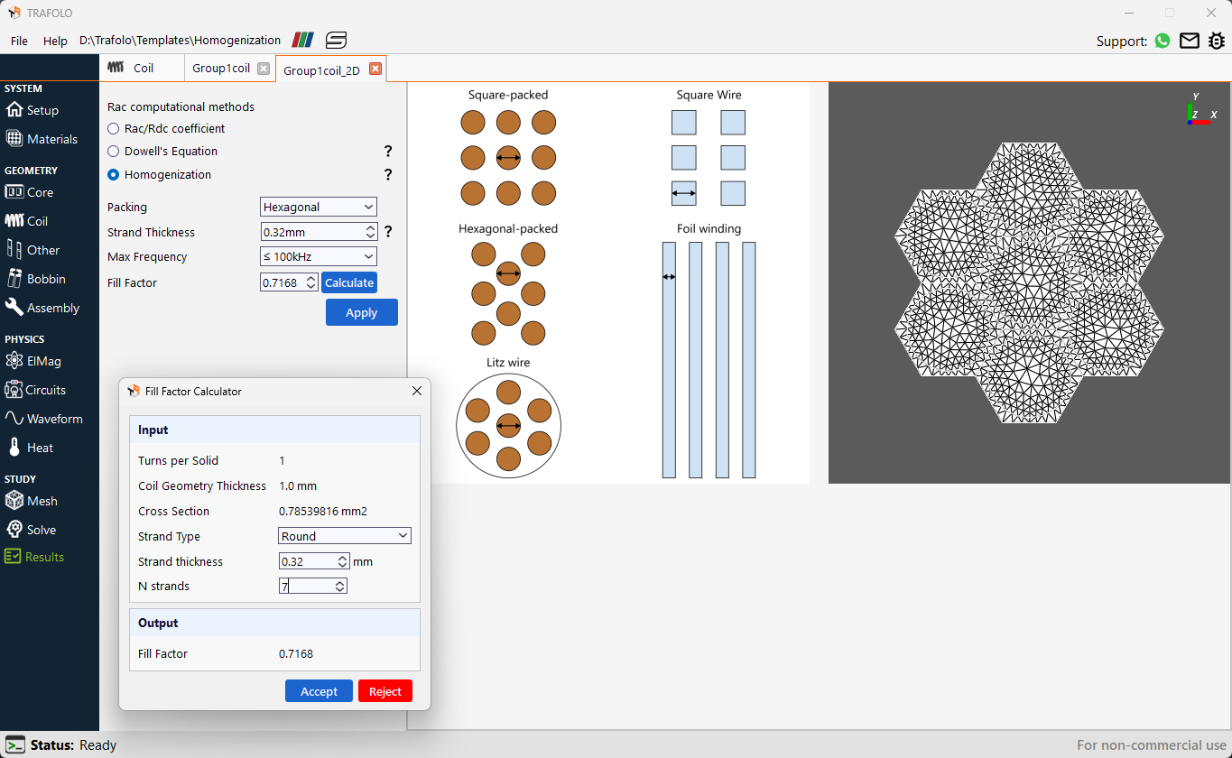
12. From the Rac coefficient methods, select Homogenization.
13. From the Packing dropdown list, select Hexagonal.
11. Click the Configure Wire button.
12. From the Rac coefficient methods, select Homogenization.
13. From the Packing dropdown list, select Hexagonal.
The packing structure of strands plays a crucial role in modeling litz wire behavior. A hexagonal arrangement of the strands closely represents the twisted structure of the litz wire. 14. In the Strand Thickness text field, enter the strand diameter of 0.32 mm. 15. From the Max Frequency dropdown list, set the operating frequency range as ≤ 100 kHz.
This will generate a 2D mesh for litz parameter calculation with sufficient refinement up to this frequency. 16. To calculate the Fill Factor, click the Calculate button. Enter the data as per the table below and click the Accept button.
| Strand Type | Strand Thickness (mm) | Number of strands per turn (N strand) |
|---|---|---|
| Round | 0.32 | 7 |
-
Click the Apply button.
 17. To streamline the process, create Group2coil by duplicating and modifying Group1coil.
Begin by navigating back to the Coil tab and selecting the Copy icon next to Group1coil. Group2coil will be created. 18. Next, click the Open in new tab icon and change the translation along the y-axis to -0.625 mm in the Rotation and Translation section. 19. Click the Apply button.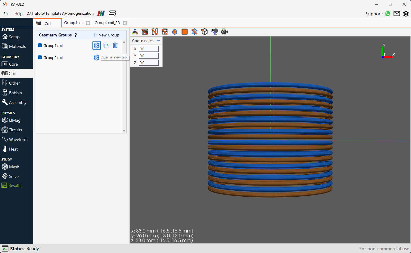
Assembly
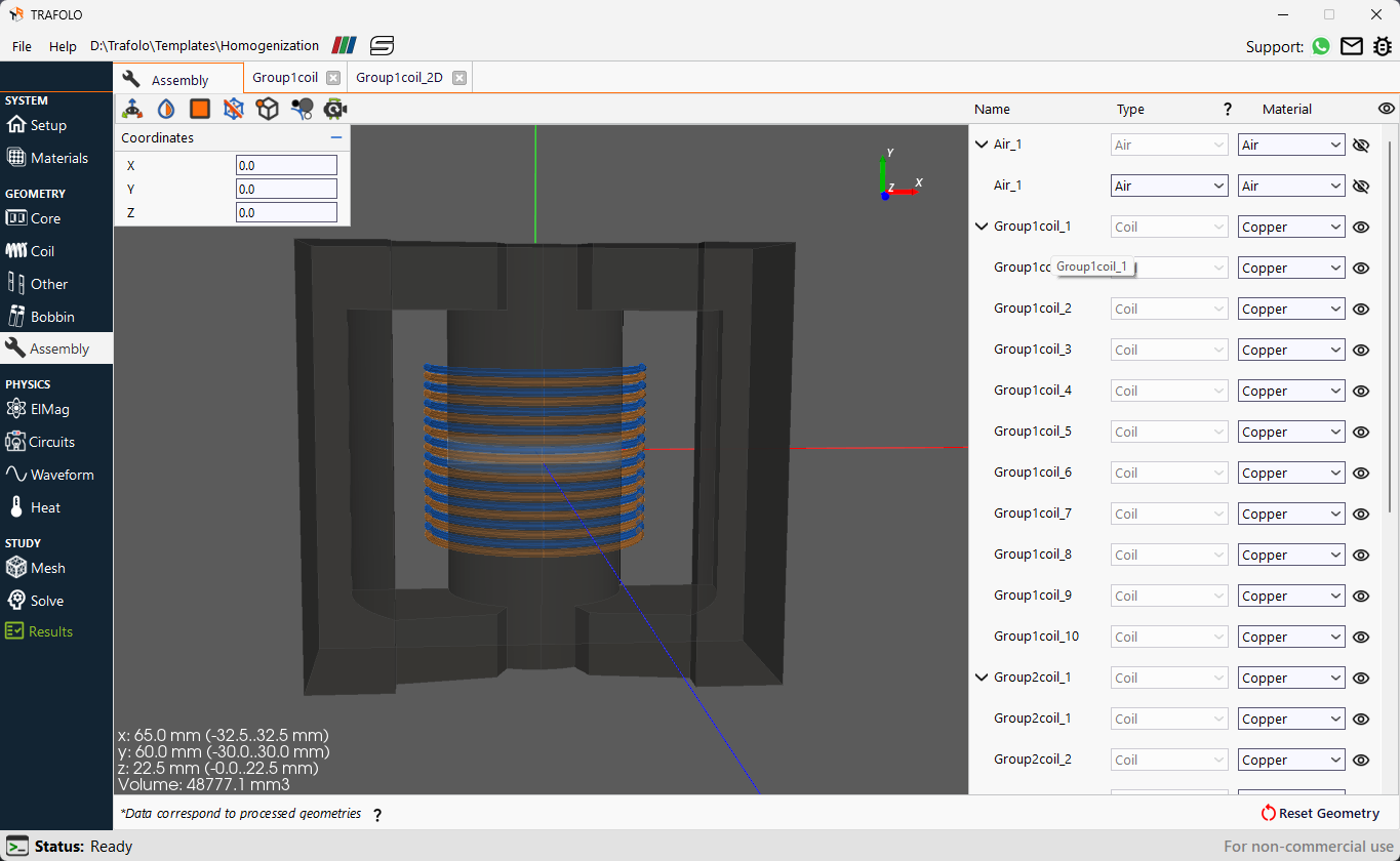
- Click the Assembly tab from the Model Builder.
- Click the Assemble Geometry button. The assembled geometry will be displayed.
EIMag
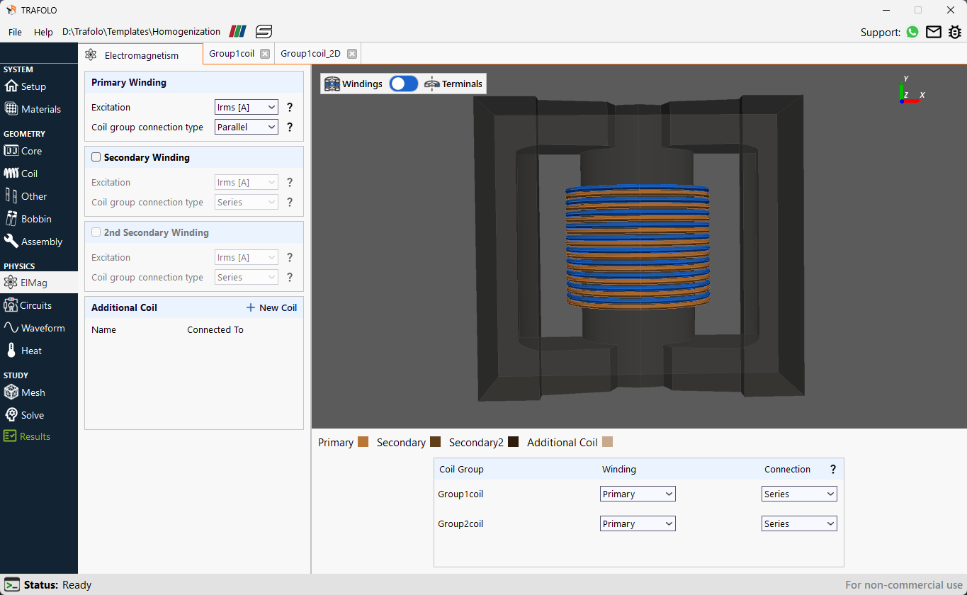
- Open the EIMag tab from the Model Builder.
- Locate the Primary Winding section.
- Set the Excitation to Irms [A], and from the dropdown menu, select Parallel for the Coil group connection type to configure Group1coil and Group2coil in parallel.
- Set the Winding and Connection for each coil group as per the table below:
| Coil Group | Winding | Connection |
| Group1coil | Primary | Series |
| Group2coil | Primary | Series |
This will connect the turns of each coil in series.
Circuit
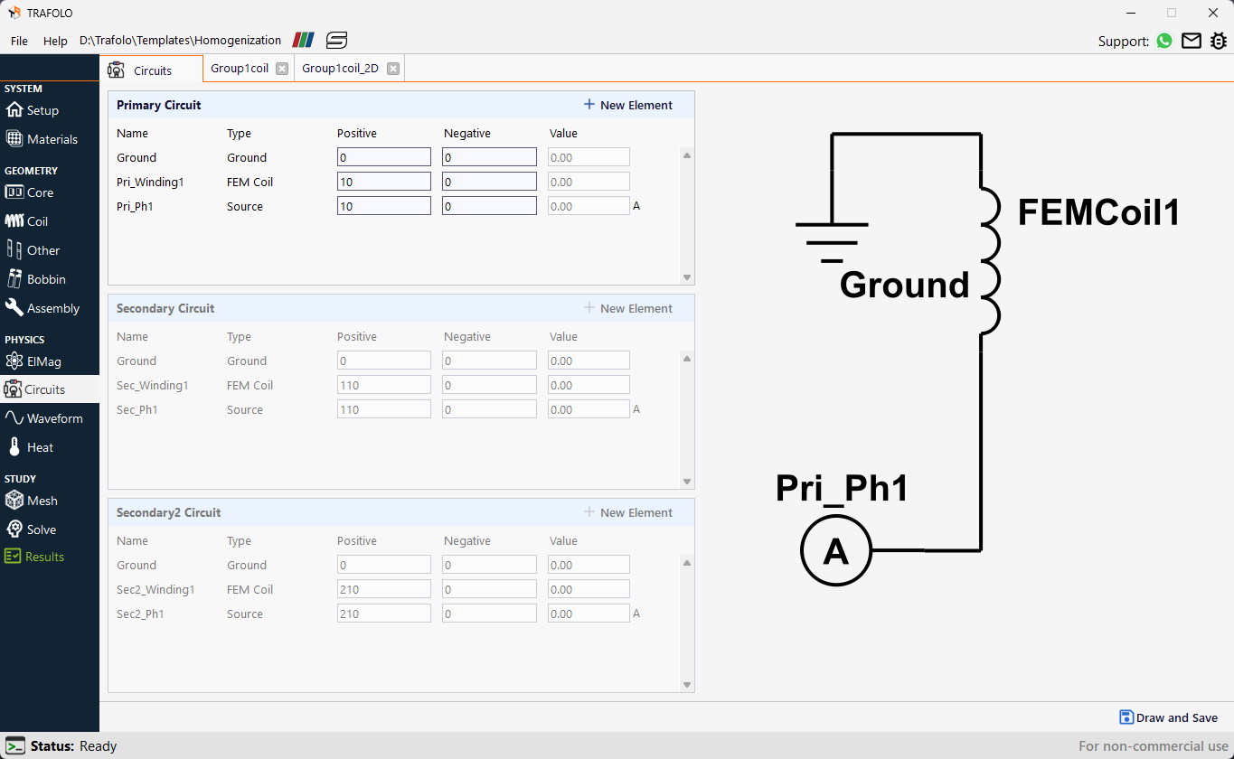
- Select the Circuits tab from the Model Builder.
- The software sets up circuits automatically, connecting FEM components and sources in series. Equal indexes for positive and negative nodes indicate that elements are connected, while different indexes denote unconnected nodes.
In this step, it is important to note that TRAFOLO has already set up the correct circuit configuration, so no further adjustments are required, and proceed directly to the next tab. - Since no circuit modifications are needed, there is no requirement to click the Draw and Save button.
Waveform
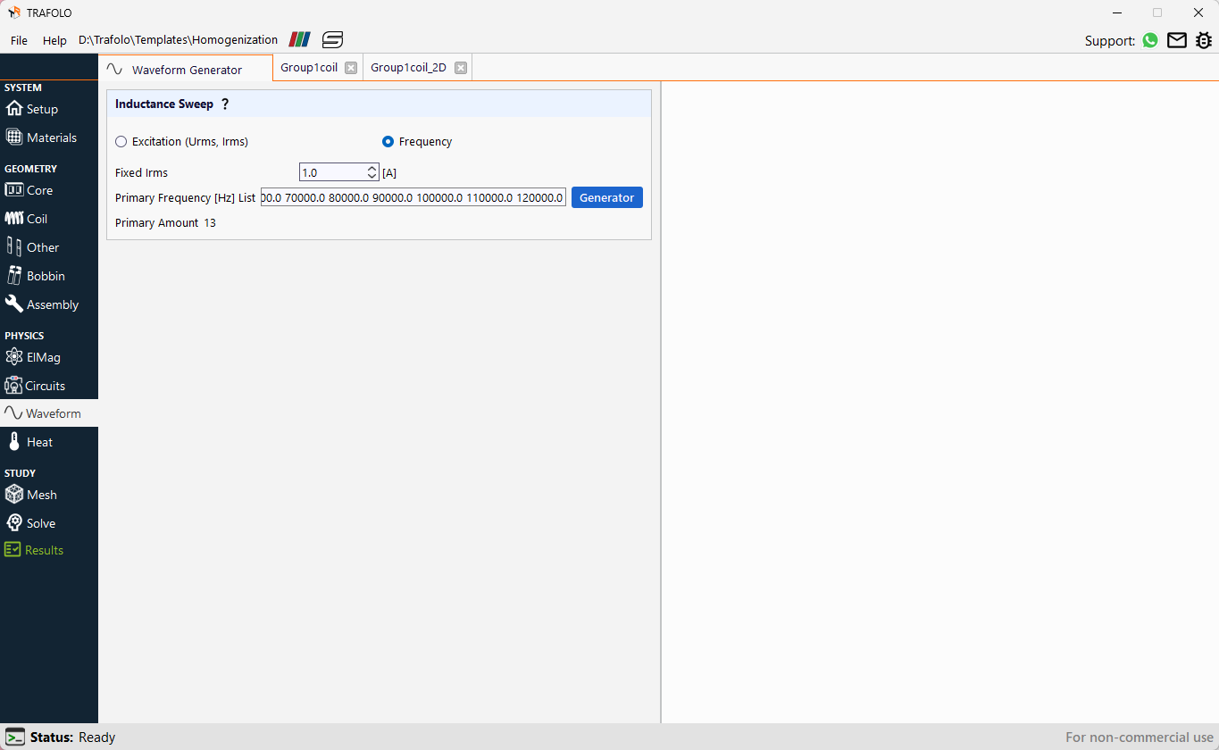
- Select the Waveform tab from the Model Builder.
- Mark the Frequency option to perform the inductance sweep across different frequencies.
- Set the Fixed Irms value to 1.0 [A].
- Click the Generator button next to the Primary Frequency [Hz] List.
- Set the Step to 10000.0 and Max to 120000.0.
- Click the Accept button.
- Also, add 0.0 at the beginning of the sequence to analyze the results at DC value.
Heat
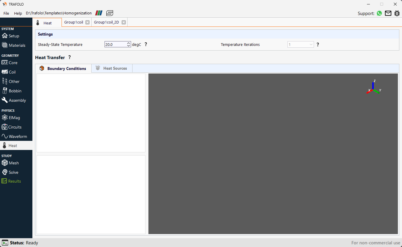
- Select the Heat tab from the Model Builder.
Although the heat simulation is disabled in the Setup, setting the temperature is still necessary to define material properties, such as the temperature-dependent electrical conductivity of copper. This temperature will also be used when calculating the homogenized properties of litz wire. - In the Settings section, enter 20.0 °C as the Steady-State Temperature.
Mesh
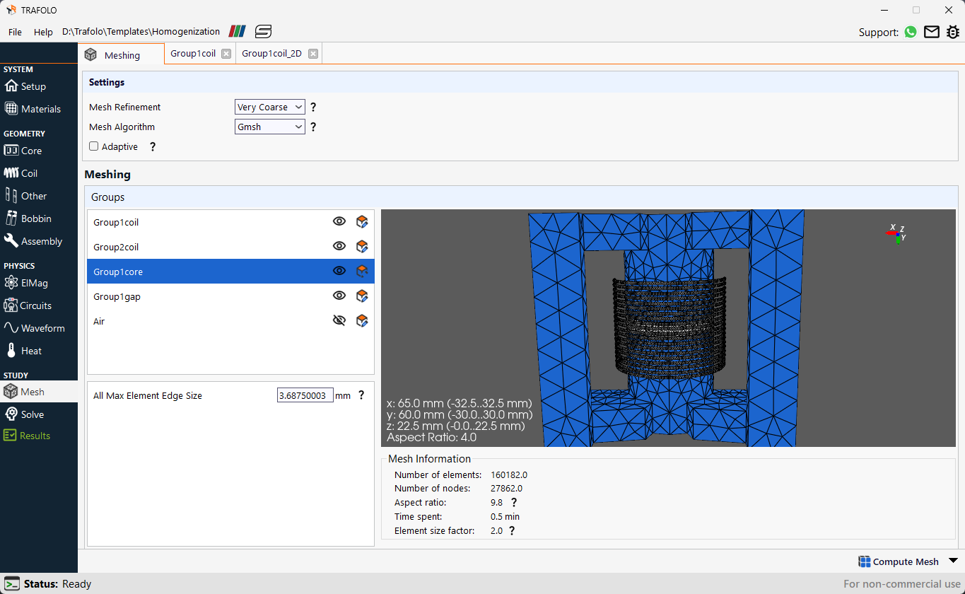
- From the Model Builder, click on the Mesh tab.
- Under the Settings section, from the Mesh Refinement dropdown list, select Very Coarse.
- Set the Mesh Algorithm to Gmsh from the dropdown list. This more robust algorithm enables the generation of coarser meshes.
- Click the mesh corresponding to each geometry group and adjust the mesh refinement by specifying the All Max Element Edge Size (mm) value according to the table below:
| Coil group | Group1coil | Group2coil | Group1core | Group1gap |
|---|---|---|---|---|
| All Max Element Edge Size (mm) | 0.25 | 0.25 | 3.69 | 0.5 |
- Click the Evaluate Mesh button followed by the Compute Mesh button.
Solve
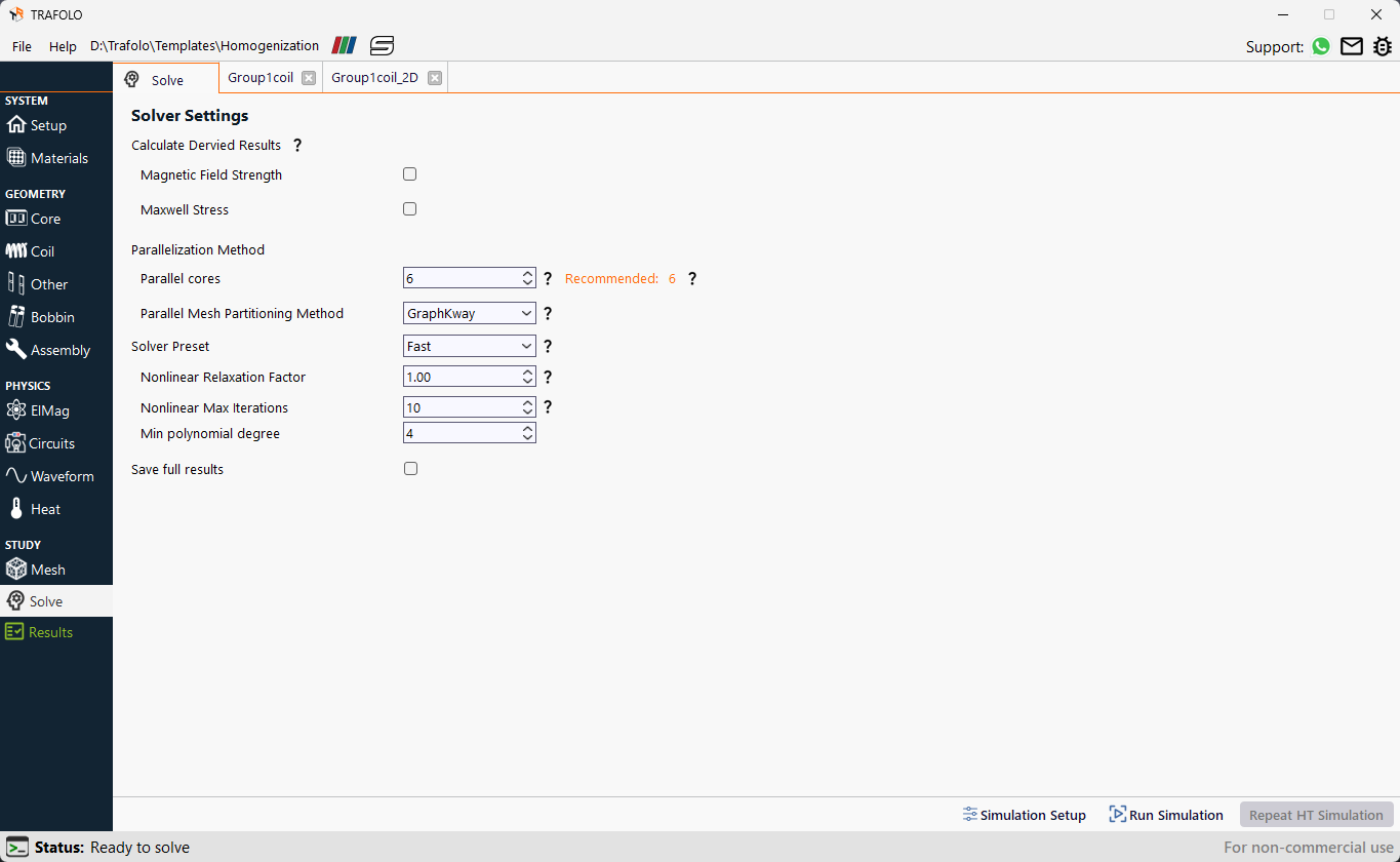
- From the Model Builder, click on the Solve tab.
- Click on the Simulation Setup button, followed by the Run Simulation button.
Results and Discussion
- From the Model Builder, click on the Results tab.
- Click on the Summary tab to get the average values of various parameters.
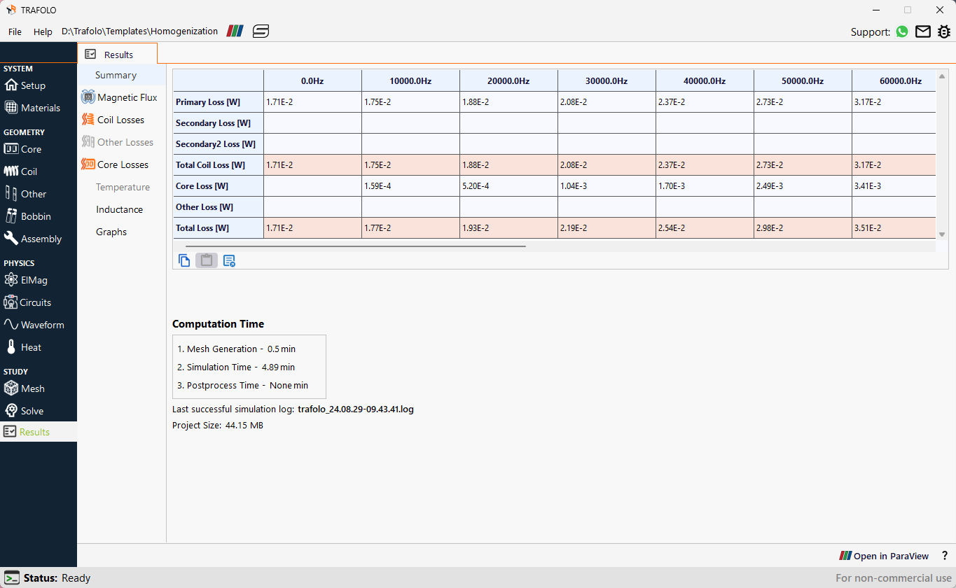
The summary indicates that as frequency increases from 0 Hz to 120 kHz with a fixed current excitation, copper losses steadily rise, marking a fourfold increase. Core losses, minimal at lower frequencies, begin to grow substantially beyond 50 kHz. The total losses primarily follow the behavior of coil losses, with core losses contributing noticeably only at frequencies above 80 kHz.
3. Additionally, the user can switch between the Results tabs to visualize the processed results, such as inductance values, winding resistance, and 3D distributions of magnetic flux density and losses.
Upon analyzing the frequency steps, it is clear that the magnetic flux distribution remains consistent throughout most of the frequency range.
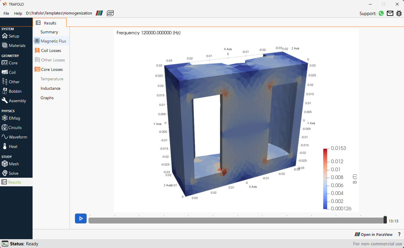
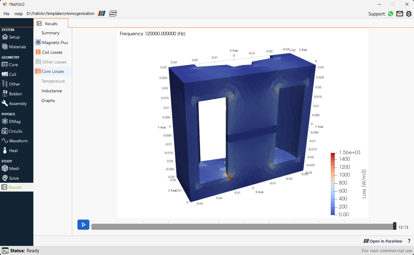
At higher frequencies, core losses become more pronounced due to the increased eddy currents resulting from skin and proximity effects. Nevertheless, these core losses remain significantly lower than the losses experienced in the coil.
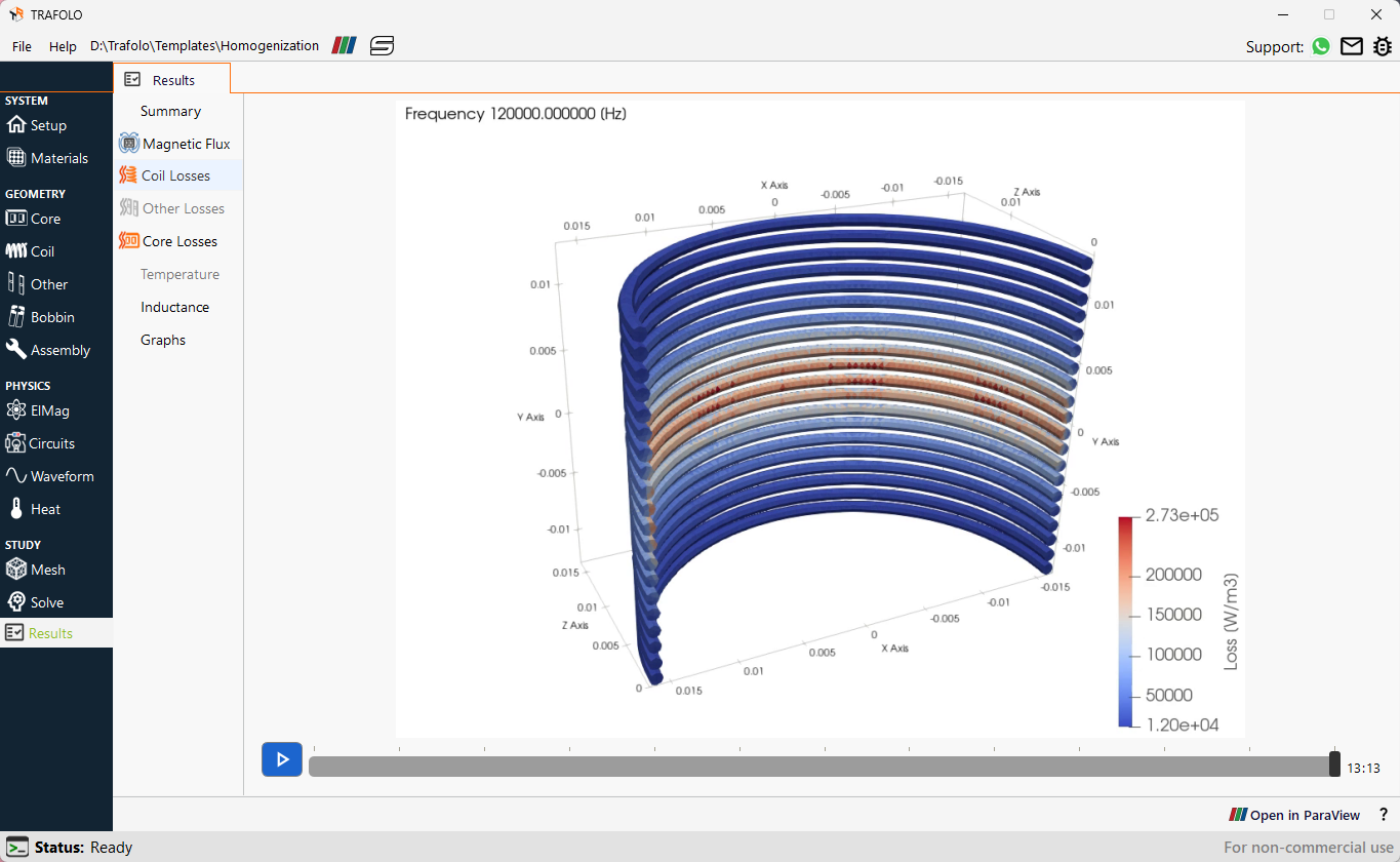
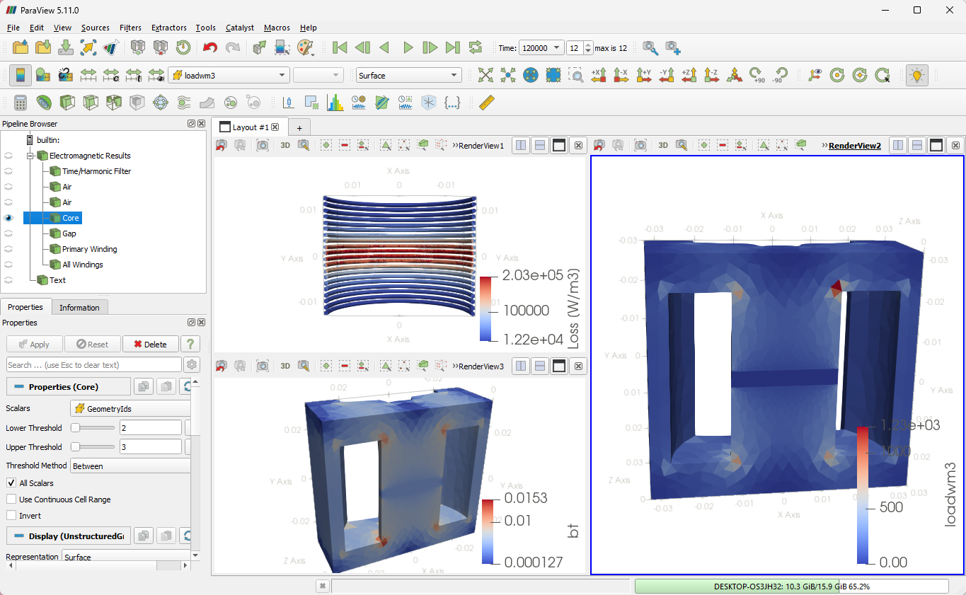
While litz wire effectively reduces losses due to the skin effect, coil losses tend to rise with frequency primarily because of the increased proximity effect, leading to an increase in effective resistance. Higher losses can be observed in the winding around the air gap region due to the proximity effect caused by the fringing flux. The circulating currents, which arise from imperfect parallelism and mutual inductance between individual litz wire strands or bundles, also contribute to the losses.
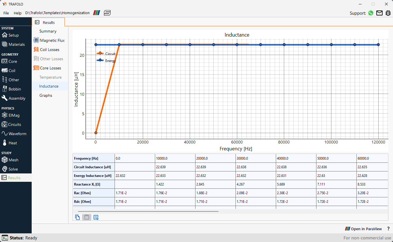
TRAFOLO calculates inductance using the Energy Method and the Circuit Method. The Energy Method calculates inductance by evaluating the magnetic field energy within the domain. In contrast, the Circuit Method calculates inductance by dividing the complex impedance by the angular frequency of the circuit. Since the frequency starts from zero, the inductance initially exhibits a gradual increase in value in this method. Despite this initial variation, both methods yield consistent results, showing that the inductance remains nearly constant across the evaluated frequency range.
The increase in reactance from 1.422 Ω at 0 Hz to 17.057 Ω at 120 kHz is linear, correlating directly with frequency increase.
The increase in inductive reactance primarily drives the initial rise in the quality factor (Q) as frequency increases. Since reactance is proportional to frequency, it grows steadily in the lower frequency range, while the AC resistance remains comparatively small. This results in a rising Q factor, as the inductive reactance dominates over resistive losses. The Q factor reaches its maximum at around 50 kHz, indicating the frequency at which the inductor operates most efficiently. Beyond this point, however, the AC resistance increases more significantly due to frequency-dependent effects like skin and proximity effects in the litz wire. As a result, the losses start to outweigh the gains from increased reactance, leading to a gradual decline in the Q factor at higher frequencies.
4. Click the Open in ParaView button to open simulation results in post-processing software. It allows manipulation with results, changing color schemes, making slices, and doing any other manipulations with results.
ParaView has been used for detailed visualization and analysis of the flux density and loss distribution, as shown in the accompanying figures.
 5. The results obtained from the TRAFOLO simulations show a strong correlation with the measured AC resistance values provided in Otomo et al.'s conference paper. The comparison plot shows that TRAFOLO's predictions closely follow the measured data across the entire frequency spectrum with minimal deviation.
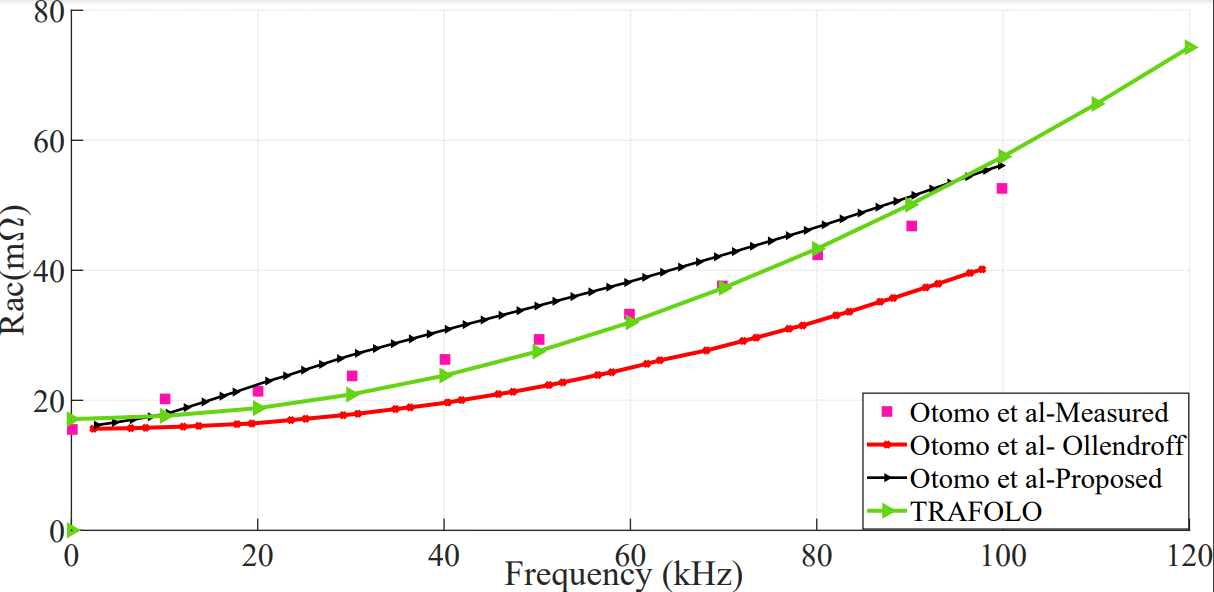
The simulation took less than 5 minutes for 13 frequency points on 10 CPU cores. It indicates that homogenization significantly reduces computational load by minimizing the number of elements needed in the mesh. This makes it faster and more scalable for modeling complex systems, such as gapped inductors and transformers, where it would be impractical to model every strand individually. Additionally, focusing on averaged properties still provides valuable insights into important parameters like resistance, inductance, and losses while maintaining accuracy.