Copy of Processing Simulation Results in ParaView

TRAFOLO automatically post-processes the most commonly used results upon successfully completing the simulation, making them available in the Results tab.
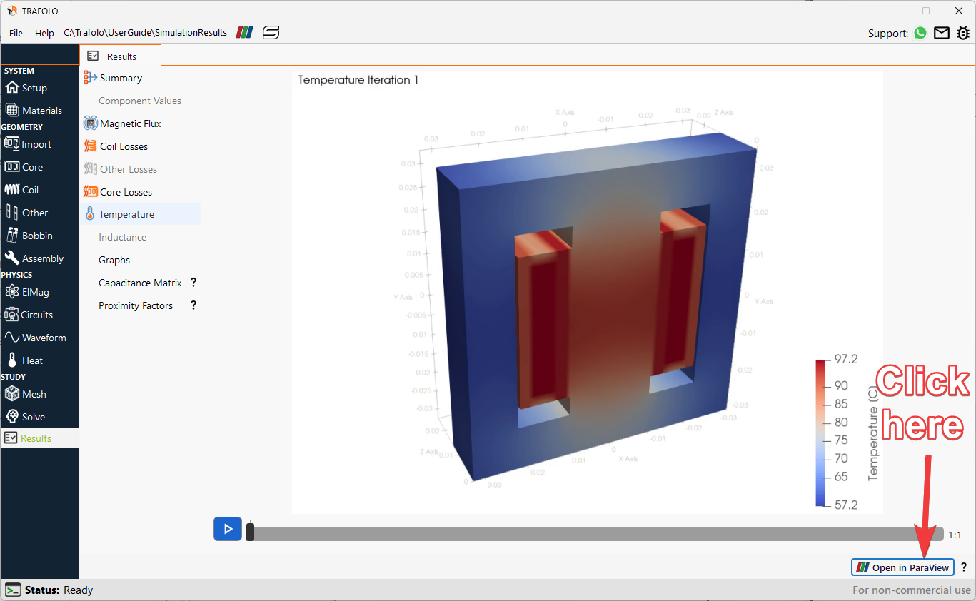
For a more in-depth analysis, users can open simulation results in ParaView by clicking the Open in ParaView button located in the bottom corner of the Results tab. This will launch ParaView and automatically load pre-configured scripts to visualize key results.

Note that ParaView will only open if full simulation results are available. In template-based or “save-as” copied cases, full results may not be stored to conserve disk space.

Alternatively, users can manually launch ParaView and load the h.pvd and load.pvd files from the results folder for post-processing, but in this case, all visualization filters must be set up manually.

Structure of Results in ParaView

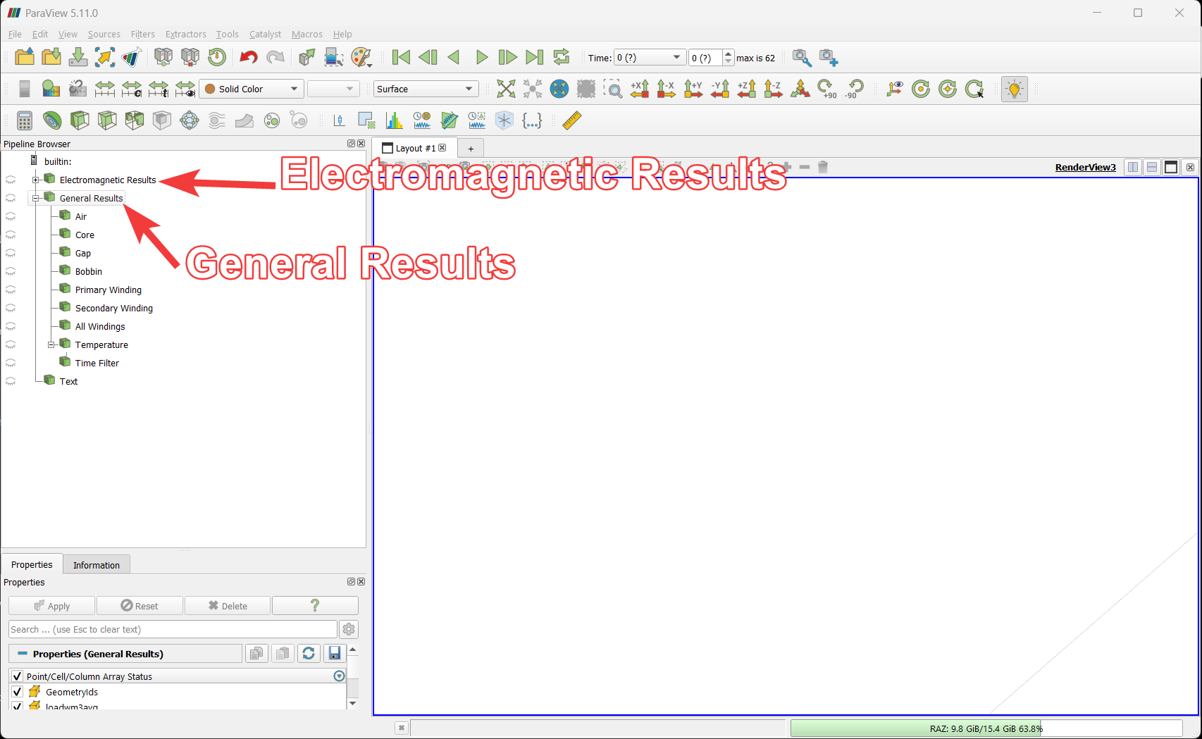
Simulation results that are opened through TRAFOLO are organized into two main categories:

1. Electromagnetic Results – These are time- or harmonics-dependent results, including current distributions, magnetic flux densities, losses, and other field values across different time steps or harmonic frequencies.
2. General Results – These are time-averaged or harmonic-summed values. They include thermal simulation outputs (if enabled), averaged losses for transient simulations, and summed fields (e.g., flux, losses) for harmonic simulations.

General Results are only available for Transient and Harmonic simulation types.

When opening results in ParaView, both Electromagnetic and General Results are loaded into the Pipeline Browser. TRAFOLO then runs a post-processing script that automatically applies relevant visualization Filters.

Visualizing Results

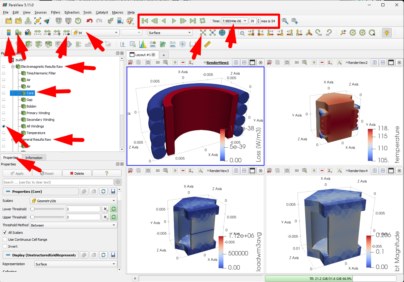
1. Enable Electromagnetics Results (by clicking on the eye icons “👁”) filters in the ParaView tabto visualize entire geometry.
2. Specific geometry can be selected and with help of filters, different result parameters can be visualised. Figure below shows visualisation of Magnetic Flux distribution for Core geometry.

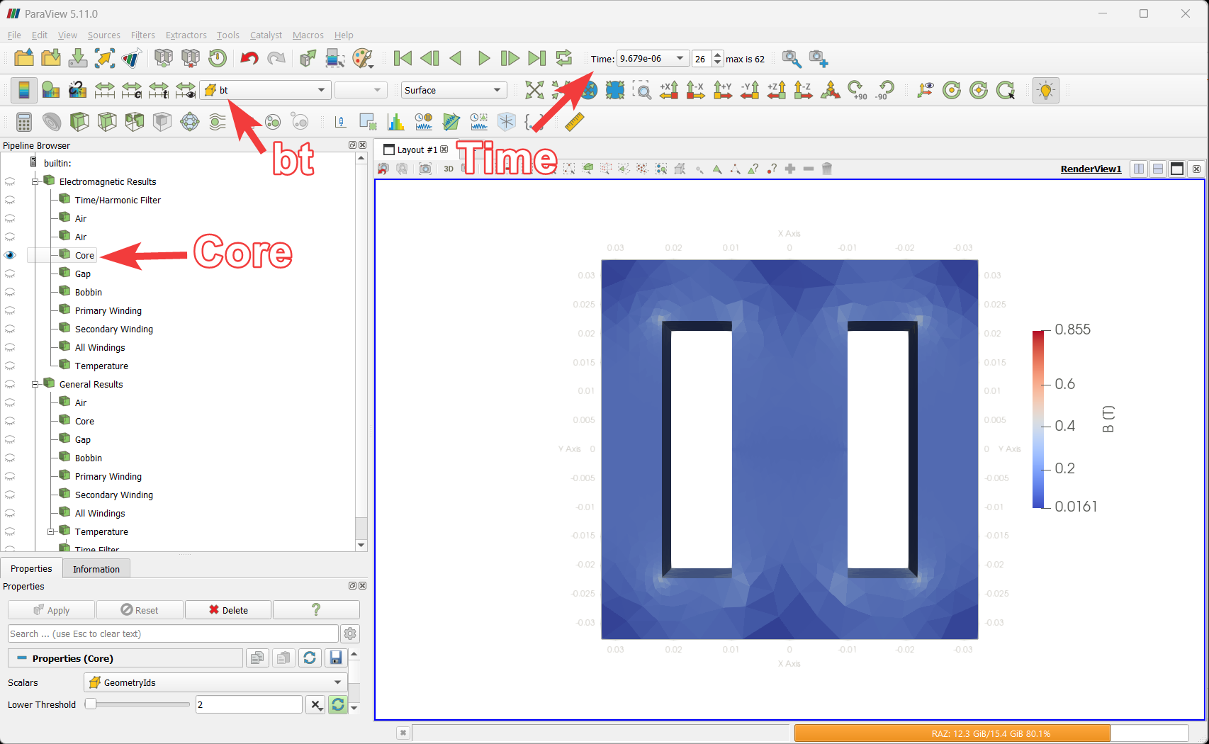
1. Similarly, other parameters such as current density, load, loss factor, magnetic flux can be visualised for relevant structures/parts of the simulation setup.
2. Click on the Hover Cells On buttonin the render toolbar, then hover over Core to see field values.

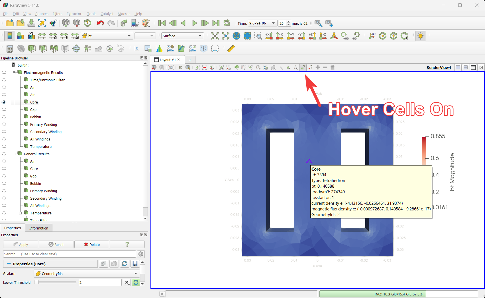
The feature Hover Cells On shows the instantaneous attribute values for one particular cell. However, for a more informative and comprehensive view,it is recommended to visualize these values over the entire simulation time.This can be achieved using the Plot Selection Over Time filter, which is explained in the following sections of this guide.

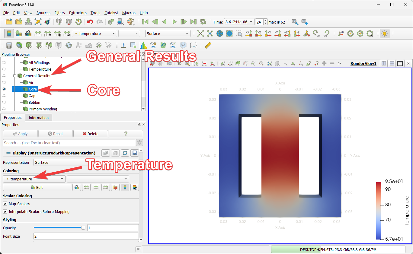
1. Furthermore, in General Results branch, we can visualise temperature for the same Core as well.

Extracting Results as Graphs

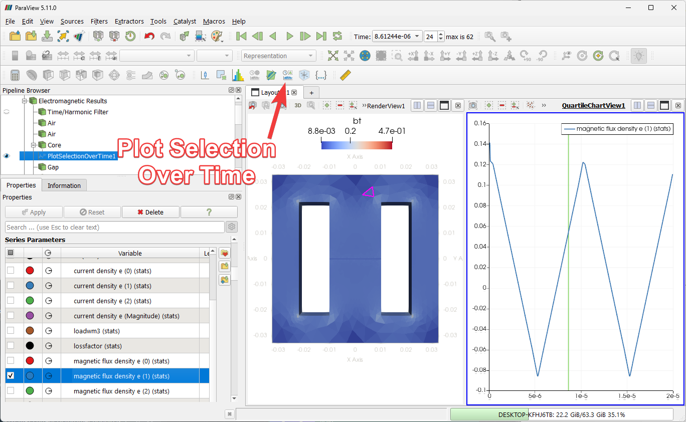
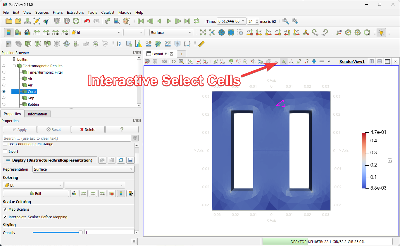
1. Select the option Interactive Select Cells On and click on a desired cell location. The selected cell will be highlighted as shown below.

1. Select Plot Selection Over Time filter and click apply under the Properties column on the left side of the window.
2. Select a desired parameter under Series Parameters cell to visualise this. Here the graph for Magnetic Flux Density distribution is shown.