Autotransformer
Introduction
Autotransformers differ from conventional transformers by utilizing a shared winding for both the primary and secondary circuits. This helps in minimizing the volume of copper required, which enhances efficiency, making autotransformers particularly well-suited for applications such as high-voltage transmission systems, renewable energy integration, and industrial power distribution.
Accurate modeling is crucial for optimizing key performance parameters, including core losses, copper losses, and thermal behavior, in the design and analysis of autotransformers. Finite Element Method (FEM) simulations, such as those implemented in TRAFOLO, provide a detailed framework for evaluating these parameters.
By utilising FEM-based analysis, autotransformer designs can be refined to minimize losses, enhance efficiency, and improve reliability. This precision engineering underscores the critical role of autotransformers in modern power infrastructure
Model Description
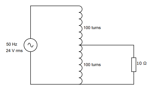
A step-down autotransformer with an EE core of E 65/32/27 is being modeled using M270-50A Cogent core material, chosen for its efficiency in optimizing magnetic performance and reducing energy losses. The transformer operates at 24V and 50Hz, with 200 turns in the primary winding. The secondary winding is tapped at 100 turns, where a 10Ω load is connected as shown in the figure.
| Core Type | Core Material | Primary Voltage | Frequency | Total Turns (Primary) | Turns (Secondary Tap) | Load |
|---|---|---|---|---|---|---|
| EE Core | M270-50A Cogent | 24V | 50 Hz | 200 | 100 | 10 Ω |
Modeling Instructions
Setup
- From the Model Builder, click the Setup tab.
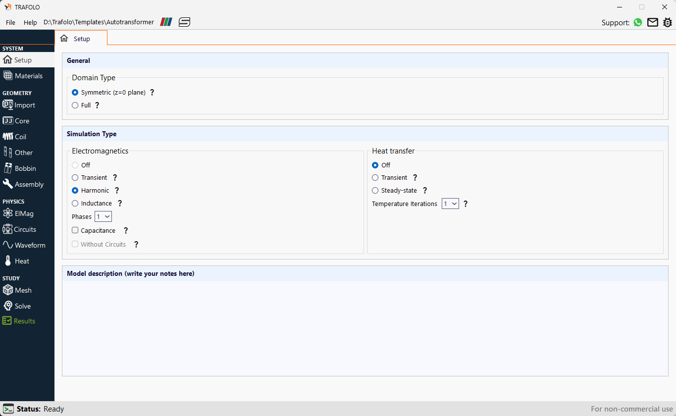
- Locate the General section and set the Domain type as Symmetric(z=0 plane).
This setting is beneficial for models with a plane of symmetry that divides the core and coil into symmetrical segments. This method ensures that the computed values reflect the complete system despite only modeling a symmetrical section. Subsequently, parameters such as voltage, resistance, losses, inductance, and other related values are appropriately scaled to represent the entire geometry accurately. - In the Simulation Type section, set Electromagnetics to Harmonic. This simulation type is suitable for sinusoidal waveforms.
- Additionally, set Heat transfer to Off as thermal effects are not a focus in this simulation.
Materials
- Select the Materials tab from the Model Builder.
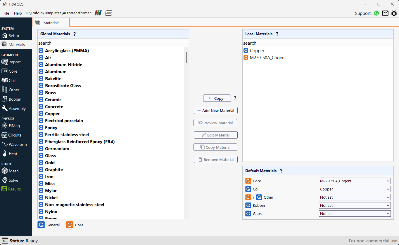
- From the Global Material section, select Copper and click the Copy button.
- Similarly, copy M270-50A_Cogent from the Global Materials section to the Local Materials section.
- In the Default Materials section, select the material type for each component from the dropdown list as per the table below:
| Component | Core | Coil | Other | Bobbin | Gaps |
| Material type | M270-50A_Cogent | Copper | Not set | Not set | Not set |
Core
- From the Model Builder, click on the Core tab.
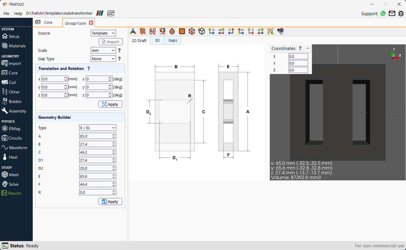
- Click the New Group button. The Group1core will be added.
- Click the Open in new tab icon “⚙“. The Group1core tab will open.
- From the Source dropdown list, select Template.
- From the Scale dropdown list, select mm.
- From the Gap Type dropdown list, select None.
- In the Geometry Builder section, set the Type to E / EL and enter the dimensions (mm) as per the table below:
| A | B | C | D1 | D2 | E | F | R |
| 65.0 | 27.4 | 44.2 | 27.4 | 20.0 | 65.6 | 44.4 | 0.0 |
- Click the Apply button.
Coil
- From the Model Builder, click on the Coil tab.
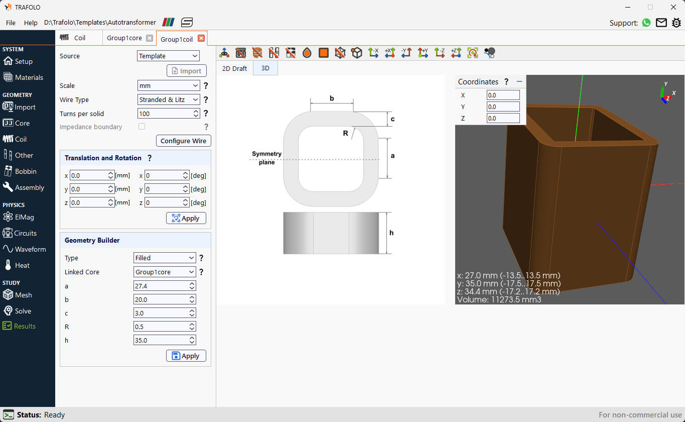
- Click the New Group tab. Group1coil will be added.
- Click the Open in new tab icon “⚙“. The Group1coil tab will open.
- From the Source dropdown list, select Template.
- From the Scale dropdown list, select mm.
- From the Wire Type dropdown list, select Stranded & Litz wire.
- Set the Turns per solid to 100.
- In the Geometry Builder section, set the Type to Filled and the Linked Core to Group1core.
- Enter the dimensions (mm) according to the table below.
| a | b | c | R | h |
|---|---|---|---|---|
| 27.4 | 20.0 | 3.0 | 0.5 | 35.0 |
- Click the Apply button.
 10. Click the Configure Wire button.
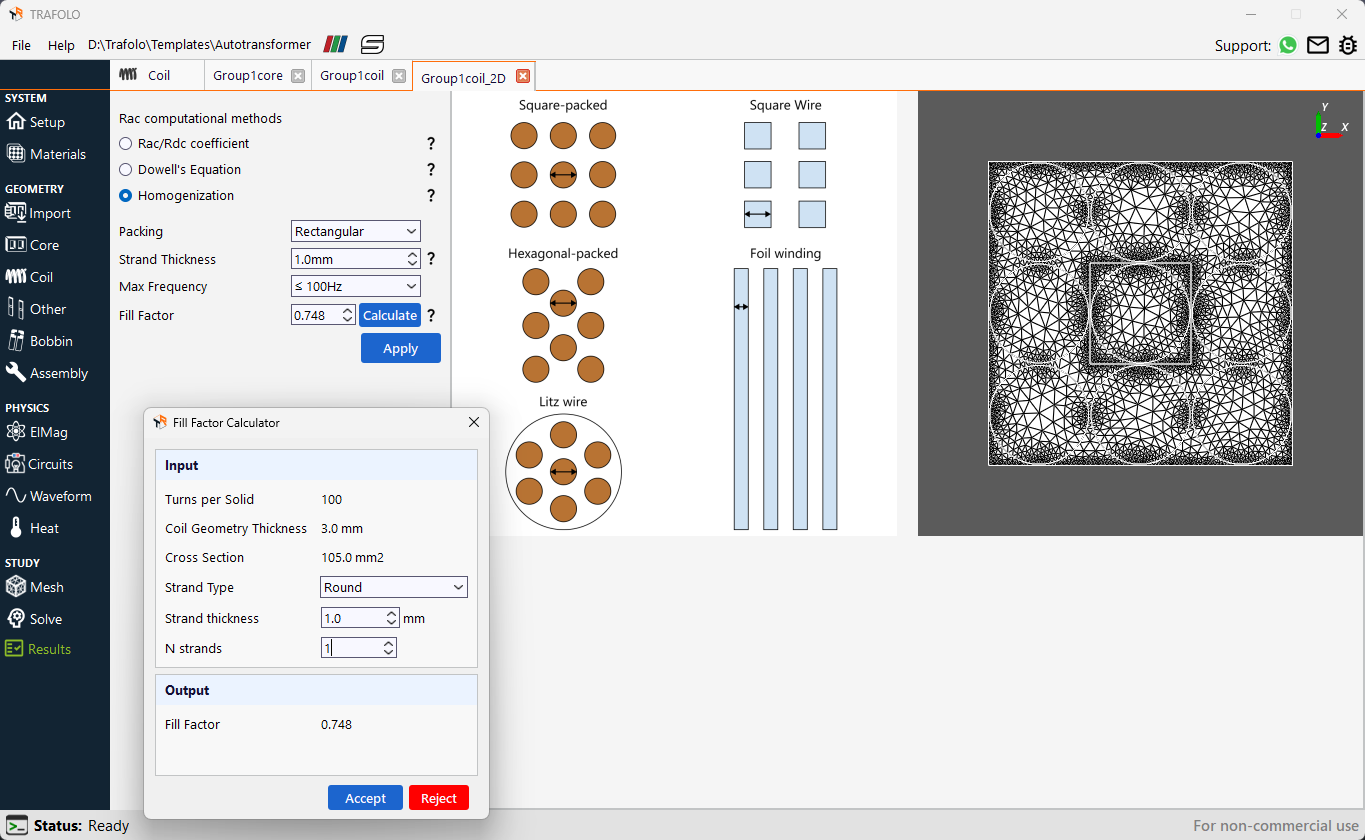
11. From the Rac coefficient methods, select Homogenization.
10. Click the Configure Wire button.
11. From the Rac coefficient methods, select Homogenization.
Since there are a hundred turns in the coil, so to save computational effort and meshing, homogenization is used.
12. From the Packing dropdown list, select Rectangular.
The packing structure of strands is required to model litz and stranded wire behavior. A rectangular arrangement of the strands closely represents the twisted structure of the stranded wire.
13. In the Strand Thickness text field, enter the strand diameter of 1.0 mm.
14. From the Max Frequency dropdown list, set the operating frequency range as ≤ 100 kHz.
This will generate a 2D mesh for litz parameter calculation with sufficient refinement up to this frequency.
15. To calculate the Fill Factor, click the Calculate button. Enter the data as per the table below and click the Accept button.
| Strand Type | Strand Thickness (mm) | Number of strands per turn (N strand) |
|---|---|---|
| Round | 1.0 mm | 1.0 |
-
Click the Apply button.
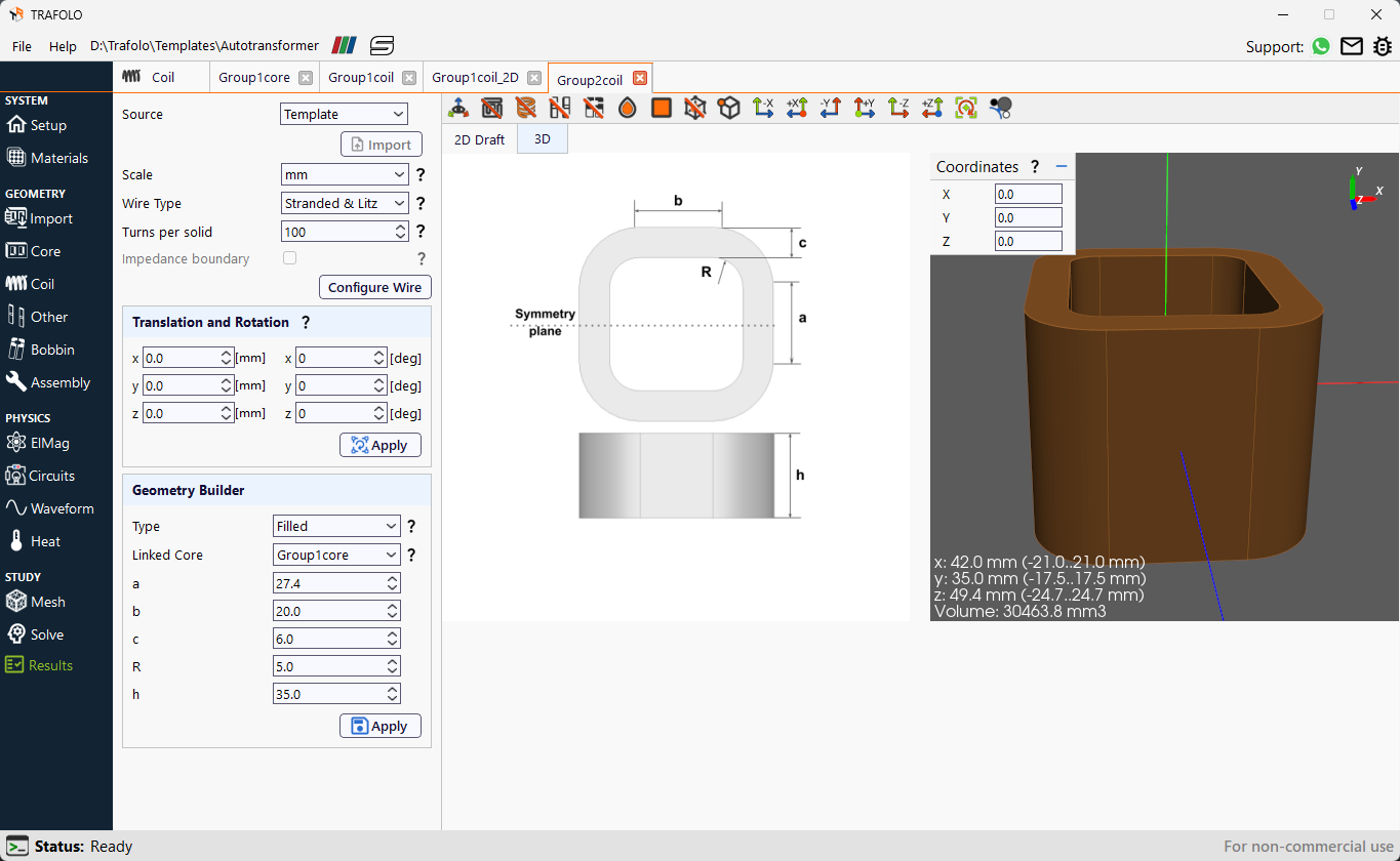
 17. Similarly, build Group2coil for secondary winding.
18. Set the Turns per solid to 100.
19. Enter the details in the Geometry Builder section as per the below table and click the Apply button.
17. Similarly, build Group2coil for secondary winding.
18. Set the Turns per solid to 100.
19. Enter the details in the Geometry Builder section as per the below table and click the Apply button.
| Type | Linked Core | a | b | c | R | h |
|---|---|---|---|---|---|---|
| Filled | Group1core | 27.4 | 20.0 | 6.0 | 5.0 | 35.0 |
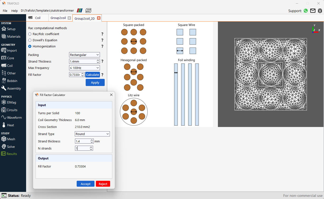
- Click the Configure Wire button.
- From the Rac coefficient methods, select Homogenization.
- From the Packing dropdown list, select Rectangular.
- In the Strand Thickness text field, enter the strand diameter of 1.4 mm.
- From the Max Frequency dropdown list, set the operating frequency range as ≤ 100 kHz.
- To calculate the Fill Factor, click the Calculate button. Enter the data as per the table below and click the Accept button.
| Strand Type | Strand Thickness (mm) | Number of strands per turn (N strand) |
|---|---|---|
| Round | 1.4 mm | 1.0 |
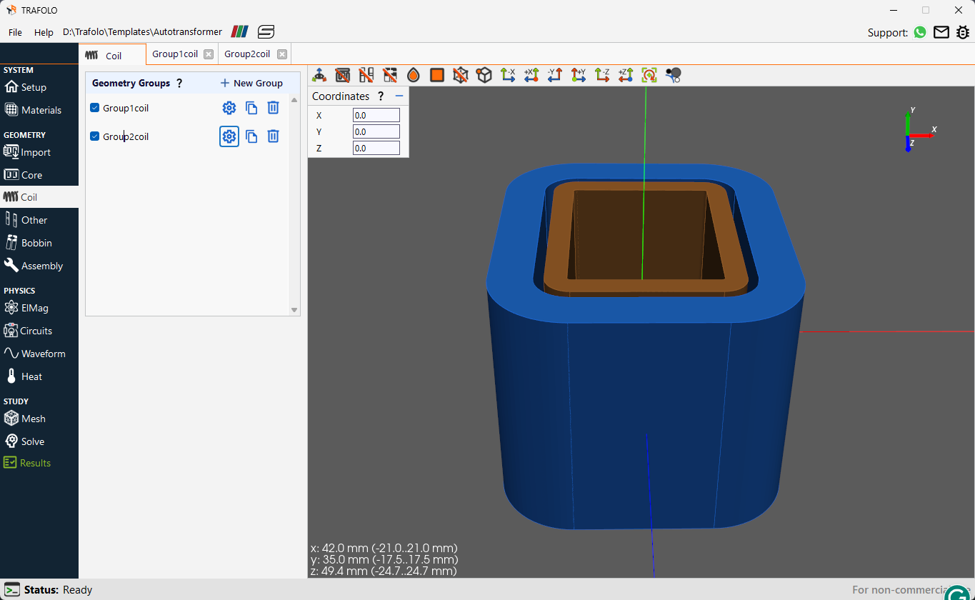
Note: In an autotransformer, power flow occurs through induction and conduction unlike in an ordinary transformer. The segment of the winding shared between the primary and secondary serves to transfer power via electrical conduction, whereas the remaining portion of the primary winding facilitates power transfer through magnetic coupling. For clarity, these two sections of the primary winding will be represented as Group2coil and Group1coil geometries, respectively.
Assembly
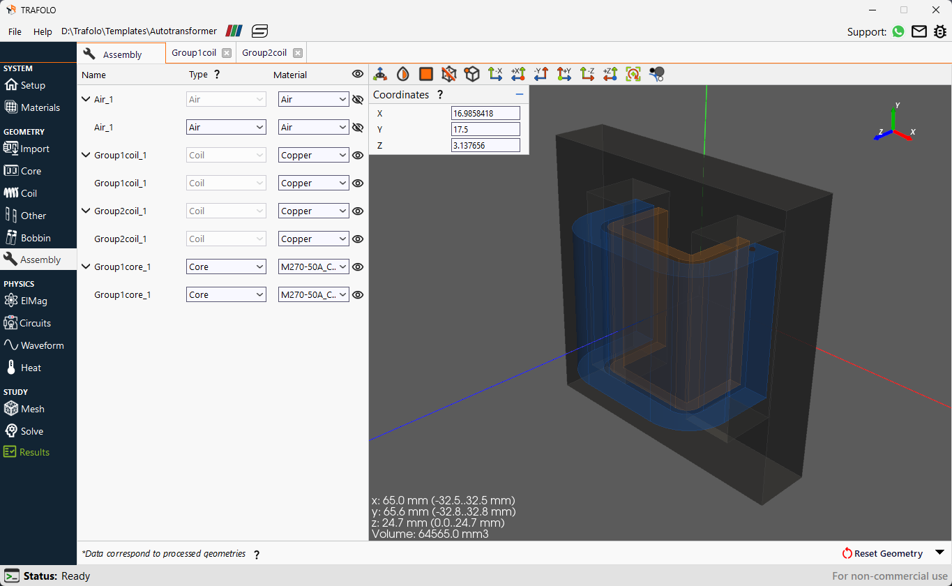
- Click the Assembly tab from the Model Builder.
- Click the Assemble Geometry button. The assembled geometry will be displayed.
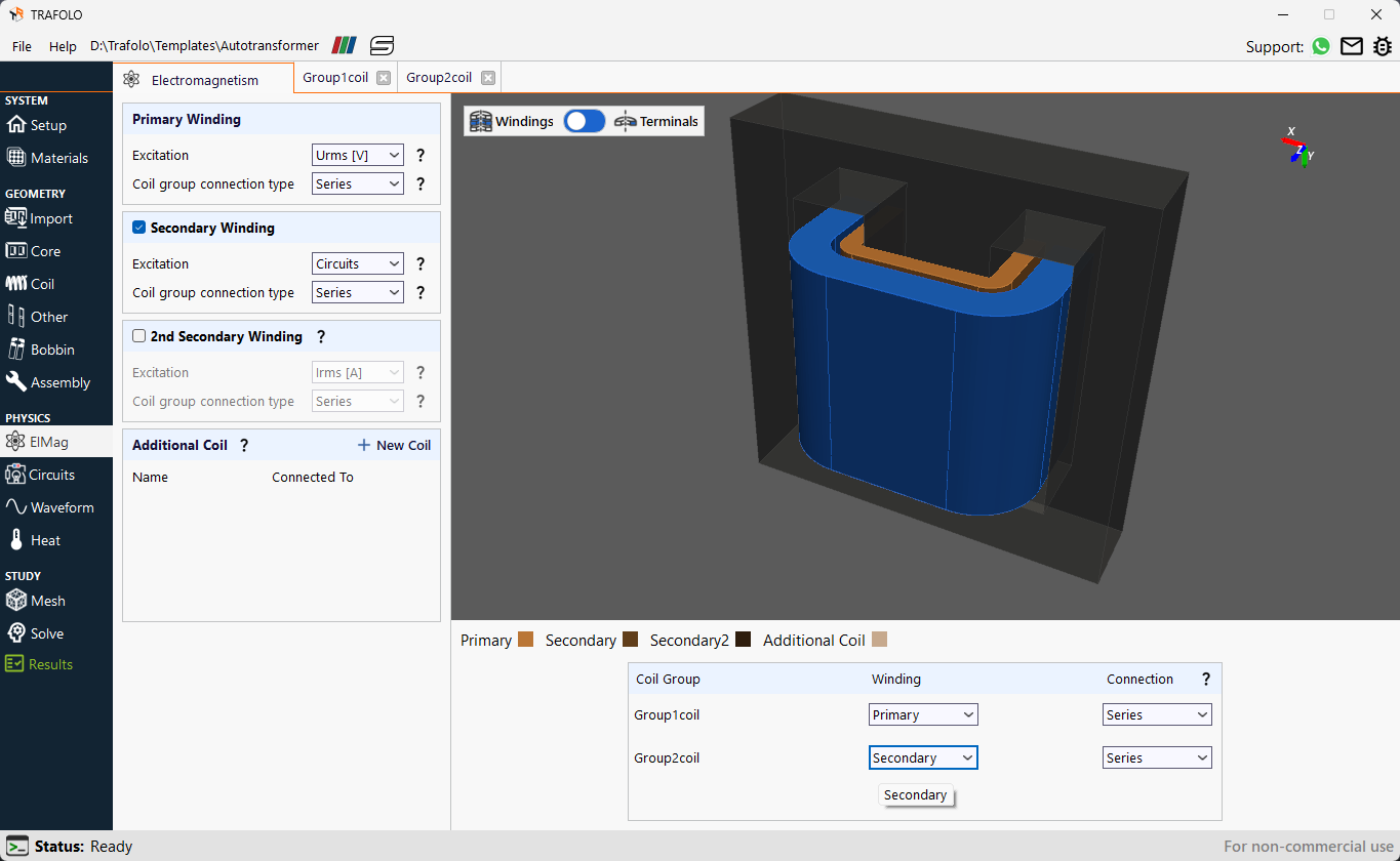
EIMag
- Open the EIMag tab from the Model Builder.
- Locate the Primary Winding section.
- Set the Excitation to Urms [V] and the Coil group connection type to Series from the dropdown list.
- Enable the Secondary Winding by checking the box.
- Set the Excitation to Circuits and the Coil group connection type to Series from the dropdown list.
- Set the Winding and Connection for each coil group as per the table below:
| Coil Group | Winding | Connection |
| Group1coil | Primary | Series |
| Group2coil | Secondary | Series |
The Group1coil and the Group2coil are designated as the primary and secondary windings in EIMag, respectively, to enable this distinction in functionality and analysis within the software.
Circuits
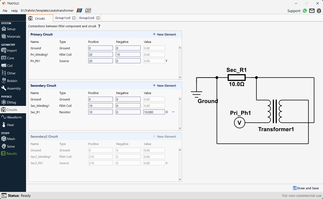
- Select the Circuits tab from the Model Builder.
- To add a load to the transformer circuit, navigate to the Secondary Circuit section and click the New Element button. Select the Resistor from the dropdown list and assign a value of 10.0 Ω.
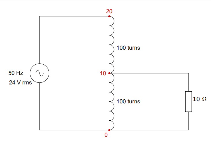 3. To build the circuit, the nodes are assigned index values to define the connectivity. Equal indexes for positive and negative nodes indicate connected elements, while different indexes imply no connection. Refer to the circuit diagram of the autotransformer with highlighted nodes and follow these steps to assign the index values:
- The primary source and the primary winding are connected to the same node. Assign this node an index value of 20.
- The common point where the secondary is tapped is assigned an index value of 10. A load (resistor) is also connected here.
- The voltage source, the secondary winding, and the load(resistor) are all connected to the reference or ground node. Assign this node an index of 0.
- Based on these connections, the table below summarizes the positive and negative index assignments for each element in both the primary and secondary circuits:
| Primary Circuit | Secondary Circuit | |||||
|---|---|---|---|---|---|---|
| Name | Ground | Pri_Winding1 | Pri_Ph1 | Ground | Sec_Windiing 1 | Sec_R1 |
| Positive index | 0 | 20 | 20 | 0 | 10 | 10 |
| Negative index | 0 | 0 | 10 | 0 | 0 | 0 |
This arrangement of nodes allows the portion of the primary winding responsible for power transfer via magnetic coupling, referred to as Pri_Winding, to be connected between the 20th and 10th indices of the winding and the portion, Sec_Windiing 1, responsible for power transfer through conduction to be connected between the 10th and 0th nodes.
- Click the Draw and Save button to confirm the setup.
Waveform
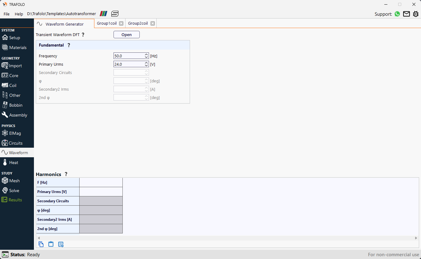
- Select the Waveform tab from the Model Builder.
- In the Fundamental section, set the Frequency and Primary Urms to 50.0 [Hz] and 24.0 [V] respectively.
Heat
- Select the Heat tab from the Model Builder.
Although the heat simulation is disabled in the Setup, setting the temperature is still necessary to define material properties, such as the temperature-dependent electrical conductivity of copper. This temperature will also be used when calculating the homogenized properties of the wire. - In the Settings section, enter 80.0 °C as the Steady-State Temperature.
Mesh
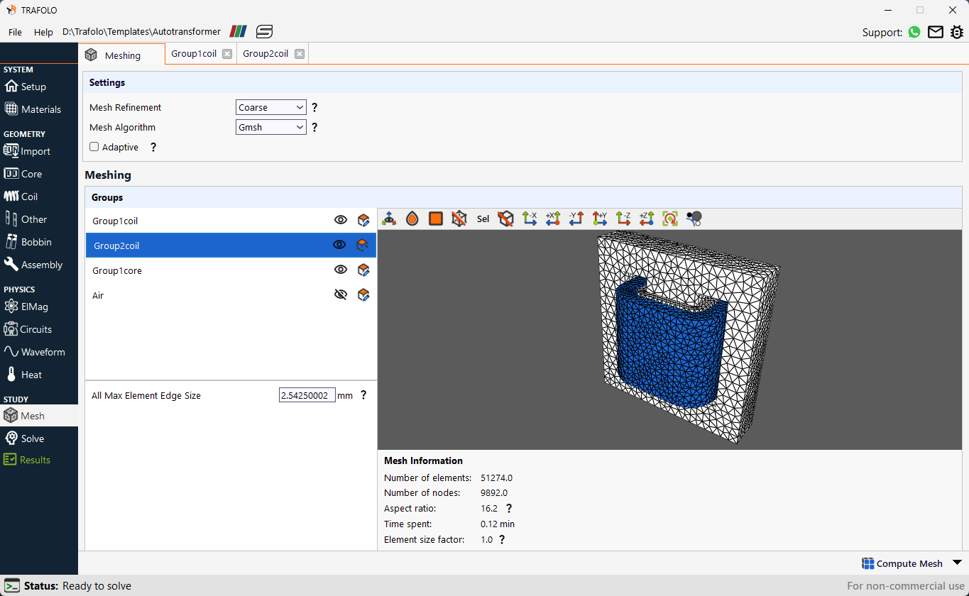
- From the Model Builder, click on the Mesh tab.
- Under the Settings section, from the Mesh Refinement dropdown list, select Coarse.
- Set the Mesh Algorithm to Gmsh from the dropdown list. This more robust algorithm enables the generation of coarser meshes.
- Click the Evaluate Mesh button followed by the Compute Mesh button.
Solve
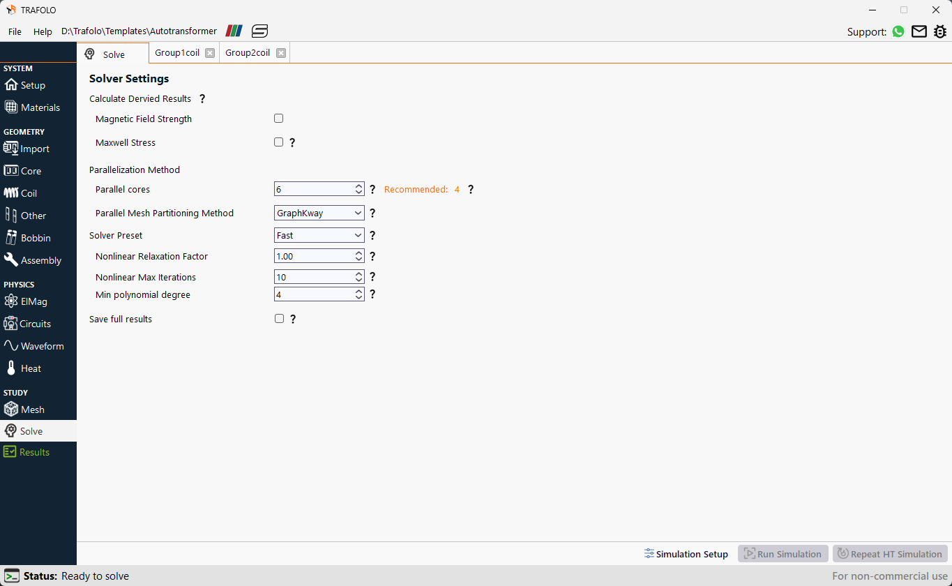
- From the Model Builder, click on the Solve tab.
- Click on the Simulation Setup button, followed by the Run Simulation button.
Results and Discussion
- From the Model Builder, click on the Results tab.
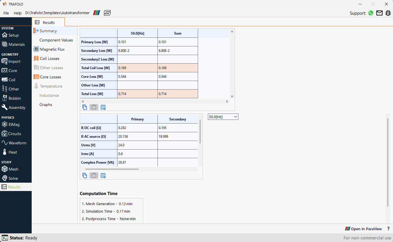
- Click on the Summary tab to get the average values of various parameters.
Upon connecting a 10-ohm load, the losses in both the windings and the core were evaluated. The transformer exhibits high efficiency, with total losses amounting to 0.714 W. Notably, core losses contribute the largest portion of these losses, indicating the dominance of magnetic material performance in overall energy dissipation.
The computation time indicates that the simulation was completed within less than a minute.
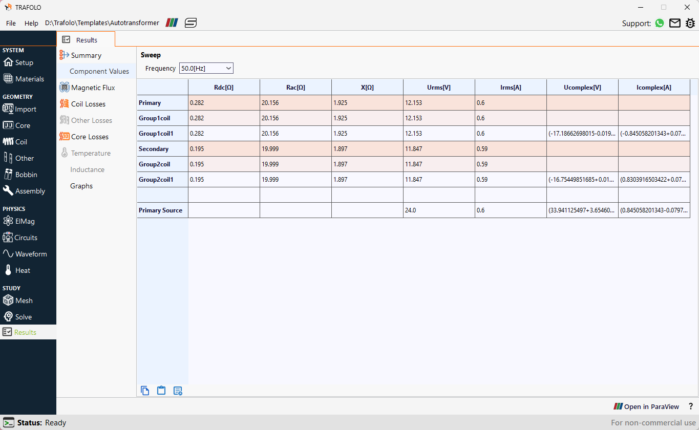
Further, various key parameters like resistances, current, complex power, etc. have been provided in detail for each component in the Component Values tab.
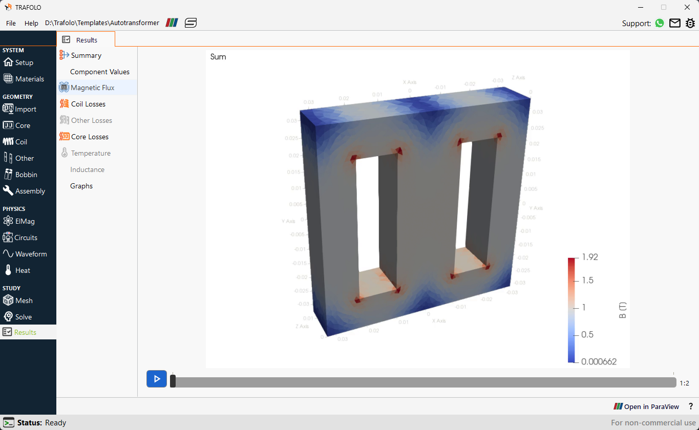
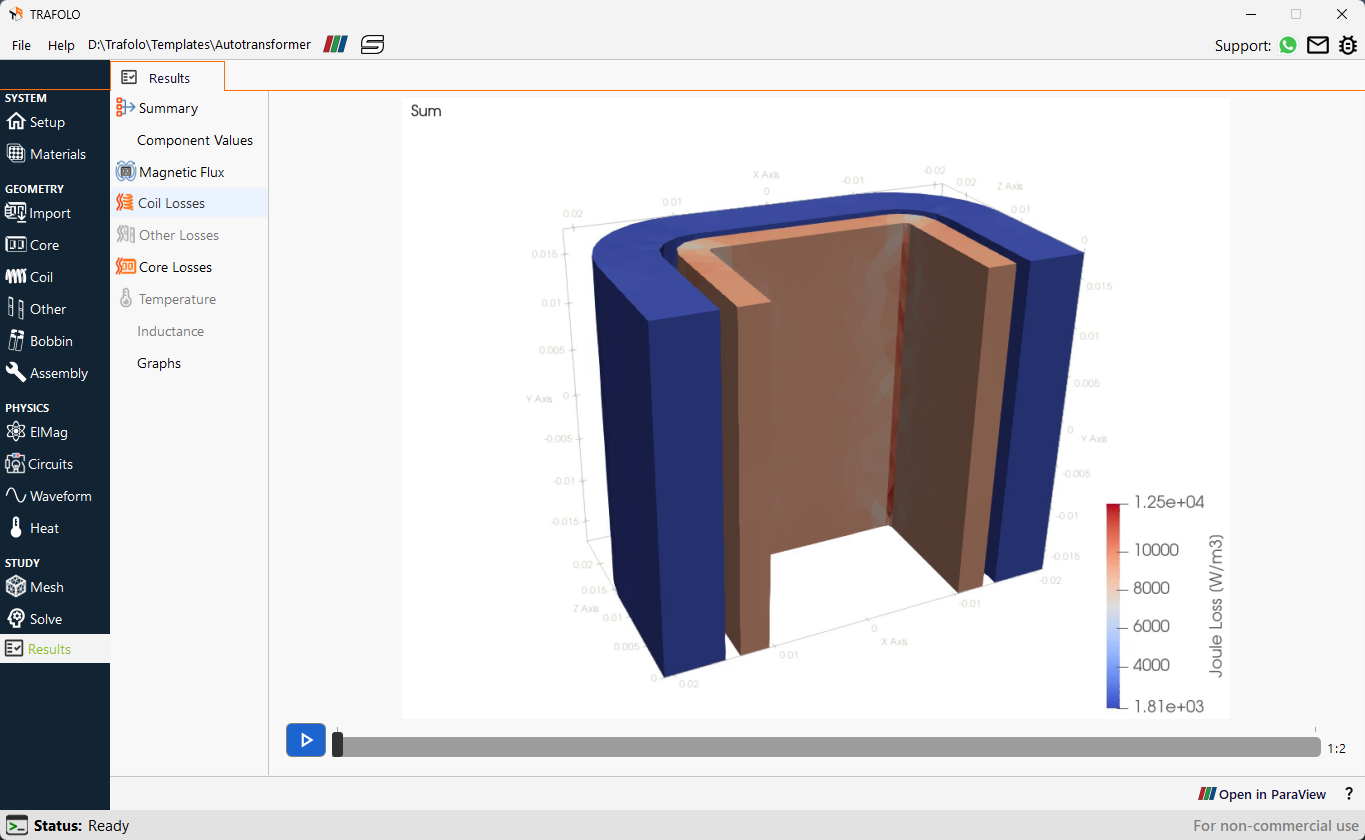
 3. Additionally, the user can switch between the Results tabs to visualize the processed results, such as 3D distributions of magnetic flux density and losses.
It can be analyzed that the flux density is almost the same in all the limbs and is below the saturation level.
Coil losses are observed to be higher in Group1coil, with lesser diameter and comparatively higher resistance.
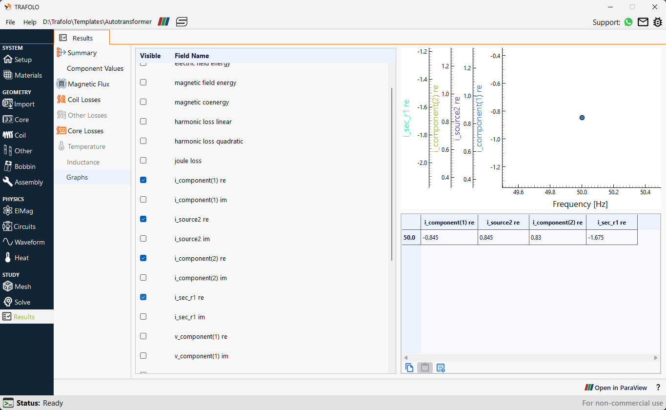
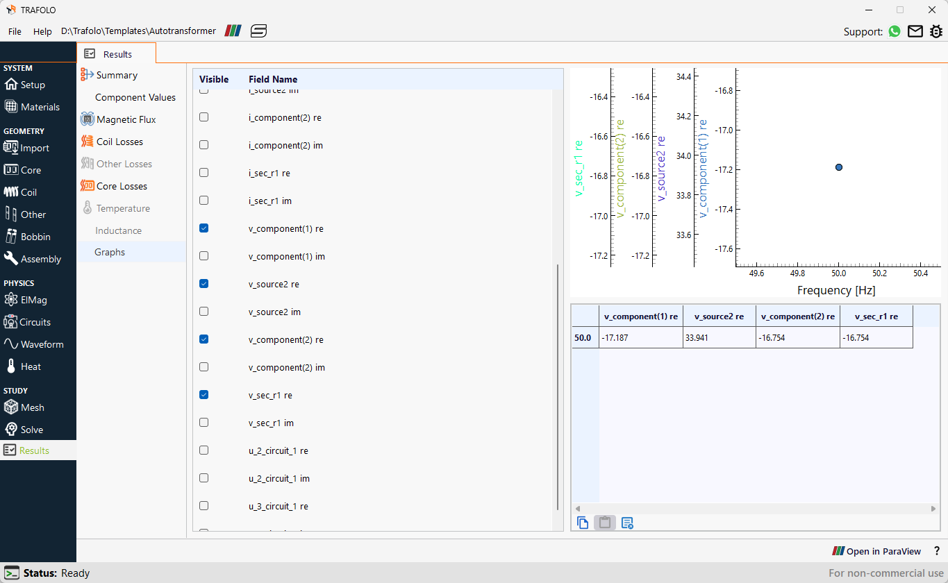
The table in the graph section of the two figures below demonstrates that the circuit adheres to Kirchoff’s current and voltage laws. This confirms that the circuit designed in the Circuit tab for the geometry is functioning effectively and producing reliable results.